Alternation Depth of Threshold Decision Lists

Podolskii, Vladimir; Prior, Morgan

doi:10.4230/LIPIcs.ICALP.2026.148

Alternation Depth of Threshold Decision Lists

Vladimir Podolskii

Tufts University, Medford, MA, USA Morgan Prior

Tufts University, Medford, MA, USA

Abstract

Linear decision lists are a computational model for Boolean functions. A linear decision list is built from a sequence of linear threshold function queries which are evaluated one by one: if a query returns true, the list outputs the value of the function, and if the answer is false, the process continues to the next query. The size of a linear decision list is the number of queries in it.

Linear decision lists form a natural and nontrivial subclass of depth-2 threshold circuits, the class of circuits that currently marks the frontier of explicit circuit lower bounds. Although some techniques for proving lower bounds against linear decision lists exist, they are quite limited, leaving important open problems unresolved. Moreover, for the related model of exact linear decision lists, no strong lower bounds are known.

We initiate the study of alternation depth of decision lists with linear threshold queries. The alternation depth is defined as the number of alternations in the sequence of output values of the decision list. We show that linear decision lists, both with bounded and unbounded weights in the threshold queries, form fine hierarchies with respect to alternation depth. A similar hierarchy exists for rectangle decision lists, the model closely related to communication complexity with NP oracles. We prove strong separations within these hierarchies and between them.

Next, we give a superpolynomial lower bound for an explicit function for exact linear decision lists of depth below $n/\log n$ . Such lower bounds were not previously known and do not follow directly from existing methods. We also establish a fine depth hierarchy for exact linear decision lists.

To prove these hierarchy separations, we use an iterative technique combined with existing techniques such as fooling sets and the analysis of blocky matrices. For the lower bound on exact linear decision lists, we combine the discrepancy method with an iterative analysis of blocky matrices.

Keywords and phrases:

linear decision lists, threshold decision lists, rectangle decision lists, threshold circuits

Category:

Track A: Algorithms, Complexity and Games

Copyright and License:

2012 ACM Subject Classification:

Theory of computation

\rightarrow

Complexity classes ; Theory of computation

\rightarrow

Oracles and decision trees ; Theory of computation

\rightarrow

Communication complexity

Related Version:

Full Version: https://eccc.weizmann.ac.il/report/2025/143/ [28]

Acknowledgements:

We would like to thank anonymous reviewers for numerous helpful comments that significantly improved the quality of the paper.

DOI:

10.4230/LIPIcs.ICALP.2026.148

Event:

53rd International Colloquium on Automata, Languages, and Programming (ICALP 2026)

Editors:

Sayan Bhattacharya, Danupon Nanongkai, Michael Benedikt, and Gabriele Puppis

Series and Publisher:

Leibniz International Proceedings in Informatics, Schloss Dagstuhl – Leibniz-Zentrum für Informatik

1 Introduction

A Boolean function $f:\{0,1\}^{n}\rightarrow\{0,1\}$ is a linear threshold function if there exist weights $w_{0},w_{1},\ldots,w_{n}\in\mathbb{Z}$ such that

f(x)=\operatorname{sgn}(w_{0}+\sum_{i=1}^{n}w_{i}x_{i}),

where we let $\operatorname{sgn}(t)=1$ for $t>0$ and $\operatorname{sgn}(t)=0$ otherwise. We denote by LTF the class of all such Boolean functions. The class $\text{\rm TC}^{0}$ of all Boolean functions computable by a polynomial-size constant-depth circuit with linear threshold functions as gates is central in circuit complexity [30, 20, 9]. Proving strong lower bounds for explicit functions even when depth is 2 is one of the main frontiers in this area [30, 20, 5]. We denote the class of functions computable by polynomial-size depth-2 threshold circuits by $\text{\rm LTF}\circ\text{\rm LTF}$ . In attempts to prove lower bounds for $\text{\rm LTF}\circ\text{\rm LTF}$ , researchers have studied weight-restricted subclasses [23, 30, 13, 10]. Define $\widehat{\text{\rm LTF}}$ ¹¹1Because $\widehat{\text{\rm LTF}}$ s can be simulated by Majority (MAJ) gates without increasing circuit depth [30], the class $\widehat{\text{\rm LTF}}$ is sometimes denoted MAJ. as the class of linear threshold functions that satisfy the additional restriction that for each $i$ , $|w_{i}|=O(\text{poly}(n))$ .

In many cases, the weight-restricted class is weaker than its unbounded analogue. For example, Myhill and Kautz [23] gave an explicit function that is in LTF but not in $\widehat{\text{\rm LTF}}$ . On the other hand, larger depth can make bounded weight classes more powerful: PARITY is computable in $\widehat{\text{\rm LTF}}\circ\widehat{\text{\rm LTF}}$ but not in LTF (see [30]). Hajnal et al. [13] proved a lower bound against $\widehat{\text{\rm LTF}}\circ\widehat{\text{\rm LTF}}$ using essentially the discrepancy method (see also [21]). Surprisingly, Goldmann, Håstad, and Razborov [10] showed that weight restrictions do not always weaken the class. Specifically, they proved $\widehat{\text{\rm LTF}}\circ\widehat{\text{\rm LTF}}=\widehat{\text{\rm LTF}}% \circ\text{\rm LTF}$ , which shows that the weights on the bottom threshold gates are irrelevant when the top weights are bounded. They further showed that $\widehat{\text{\rm LTF}}\circ\text{\rm LTF}\subsetneq\text{\rm LTF}\circ% \widehat{\text{\rm LTF}}$ , demonstrating that large weights on the top gates do increase computational power, and that $\text{\rm LTF}\circ\widehat{\text{\rm LTF}}$ is the most powerful class among depth-2 threshold circuits with bounded weights at some level.

Forster et al. [8] obtained a lower bound against $\text{\rm LTF}\circ\widehat{\text{\rm LTF}}$ using the sign-rank method, which has since become a standard lower bound technique in complexity theory [31, 7, 26]. However, Chattopadhyay and Mande [4] showed that sign-rank fails to prove lower bounds against $\text{\rm LTF}\circ\text{\rm LTF}$ : they exhibited an explicit function with large sign-rank that is computable in $\text{\rm LTF}\circ\text{\rm LTF}$ . From this, it follows that $\text{\rm LTF}\circ\widehat{\text{\rm LTF}}\subsetneq\text{\rm LTF}\circ\text{% \rm LTF}$ . Thus, the current picture of the threshold circuit hierarchy up to $\text{\rm LTF}\circ\text{\rm LTF}$ is

\widehat{\text{\rm LTF}}\subsetneq\text{\rm LTF}\subsetneq\widehat{\text{\rm LTF% }}\circ\widehat{\text{\rm LTF}}=\widehat{\text{\rm LTF}}\circ\text{\rm LTF}% \subsetneq\text{\rm LTF}\circ\widehat{\text{\rm LTF}}\subsetneq\text{\rm LTF}% \circ\text{\rm LTF}.

The challenge of proving lower bounds against $\text{\rm LTF}\circ\text{\rm LTF}$ motivates the study of other restricted computational models whose gates are threshold functions, such as linear decision lists [3, 5].

A decision list $\mathcal{L}$ of size $s$ computing a boolean function $f$ is a sequence of $\ell-1$ instructions of the form if $f_{i}(x)=a_{i}$ then output $b_{i}$ and stop, followed by the instruction output $b_{s+1}$ and stop. Here each $f_{i}$ is a query function, and $a_{i}$ and $b_{i}$ are Boolean constants. If the functions $f_{i}$ all belong to a function class $S$ , then $L$ is said to be an $S$ -decision list. A linear decision list is an $S$ -decision list with $S=\text{\rm LTF}$ . We denote the class of functions computable by a linear decision list whose size is polynomial in $n$ by LDL. It is not hard to see that $\text{\rm LDL}\subseteq\text{\rm LTF}\circ\text{\rm LTF}$ [32].

Several techniques exist for proving lower bounds on LDL size. One such technique is monochromatic rectangle size. To use this technique on a function $f:\{0,1\}^{n}\times\{0,1\}^{n}\rightarrow\{0,1\}$ , we consider its communication matrix $M_{f}$ , the $2^{n}\times 2^{n}$ matrix with entries $M_{f}[x,y]:=f(x,y)$ . A combinatorial rectangle is a set $R=A\times B$ , where $A,B\subseteq\{0,1\}^{n}$ . A combinatorial rectangle is monochromatic if $M_{f}[x,y]$ is the same for all $(x,y)\in R$ . It was established in [3] that for any product distribution $\mu\times\nu$ , if $M_{f}$ has no monochromatic combinatorial rectangle of weight greater than $w$ under the distribution $\mu\times\nu$ , then any linear decision list computing $f$ must have size at least $\frac{1}{\sqrt{w}}$ . In particular, if $f\in\text{\rm LDL}$ , $M_{f}$ has at least one large size (that is at least a polynomial fraction of $M_{f}$ ) rectangle.

Sign-rank can also be used to prove lower bounds for the size of LDLs. More specifically, it is known that if a Boolean function is computable by an LDL of size $s$ , then its communication matrix has sign-rank $O(s)$ .²²2This follows from the fact that $\text{\rm LDL}\subseteq{\text{\rm mpPTF}}$ (Lemma 20 in [6]) and the fact that functions in the class mpPTF have low sign-rank (Lemma 7 in [17]).

Despite these techniques, our ability to prove lower bounds for the class LDL is still rather limited. For example, it is unknown whether it is strictly weaker than its bounded-weight analogue, $\widehat{\text{\rm LDL}}$ [3, 6], or whether LDL is strictly weaker than the class of polynomial-size linear decision trees. Finally, while it is known that LDL is incomparable with $\widehat{\text{\rm LTF}}\circ\widehat{\text{\rm LTF}}$ , the relationship between LDL and $\text{\rm LTF}\circ\widehat{\text{\rm LTF}}$ remains unknown [3].

Another related model (although not a subclass of $\text{\rm LTF}\circ\text{\rm LTF}$ ) is the rectangle decision list, whose query functions test membership in combinatorial rectangles. Formally, let Rect denote the set of all functions $f\colon\{0,1\}^{n}\to\{0,1\}$ such that $f(x,y)=1\iff(x,y)\in R$ where $R$ is some combinatorial rectangle in $M_{f}$ . A rectangle decision list is an $S$ -decision list with $S=\text{\rm Rect}$ ; we call the class of functions computable by such a decision list Rect-DL. This class is related to those discussed above, since the rectangle size technique can be used to prove lower bounds on the length of rectangle decision lists [3, 18]. This class can also be viewed in light of its connection to the communication complexity class $\text{\rm P}^{\text{\rm NP}^{cc}}$ , which allows oracle queries to functions in $\text{\rm NP}^{cc}$ . In particular, it is known that $\text{\rm Rect}\text{\rm-DL}=\text{\rm P}^{\text{\rm NP}^{cc}}$ for quasipolynomial-sized Rect-DLs and $\text{\rm P}^{\text{\rm NP}^{cc}}$ protocol trees [25, 11].

Finally, perhaps the most intriguing subclass of $\text{\rm LTF}\circ\text{\rm LTF}$ of this flavor is ELDL, the class of decision lists whose query functions are exact threshold functions. We say a function $f:\{0,1\}^{n}\rightarrow\{0,1\}$ is an exact linear threshold function if there exist weights $w_{0},w_{1},\ldots,w_{n}\in\mathbb{Z}$ such that $f(x)=1\Leftrightarrow w_{0}+\sum_{i=1}^{n}w_{i}x_{i}=0.$ We use ELTF to denote the class of exact linear threshold functions. An exact linear decision list is an $S$ -decision list with $S=\text{\rm ELTF}$ . The class of Boolean functions computable by a polynomnial-sized exact linear decision list is denoted ELDL. It is known that ELDL contains LDL [5] and is strictly more powerful: the Block-Equality function $\text{\rm OR}_{n}\circ\text{\rm EQ}_{n}$ requires an exponential-size linear decision list, but can be computed by a polynomial-size exact linear decision list [3, 18].

Proving strong lower bounds against ELDL for an explicit function is therefore a natural intermediate step toward lower bounds for $\text{\rm LTF}\circ\text{\rm LTF}$ . However, known lower bound techniques against the class LDL do not work for ELDL. It was observed in [3] that monochromatic rectangle size does not work, as [18] showed that the Block-Equality function has no large monochromatic rectangles. Sign-rank also cannot prove lower bounds against ELDL, as [4] gave an explicit function with sign-rank $2^{\Omega(n^{1/4})}$ which is computable by a linear-size exact linear decision list.

At present, we lack techniques for proving strong lower bounds against ELDL, and more broadly for understanding threshold decision lists and depth-2 threshold circuits. This motivates the search for new methods to separate and characterize these classes.

One way to better understand linear decision lists and related computational models is to look at other parameters of these models. One of the possible parameters is the number of alternations in the outputs of the decision list. For a decision list $\mathcal{L}$ (of any type) described by the sequence

(q_{1},a_{1},b_{1}),(q_{2},a_{2},b_{2}),\ldots,(q_{s},a_{s},b_{s}),b_{s+1},

the alternation depth of $\mathcal{L}$ is equal to $|L|$ where $L:=\{i:b_{i}\neq b_{i-1}\}$ . Intuitively, we can partition the decision list into contiguous blocks of queries where the outputs $b_{i}$ are constant within each block. The alternation depth is simply the number of these blocks. When the context is clear, we often refer to “alternation depth” simply as “depth.”

Alternation depth has been studied before. It was considered as a parameter for learning algorithms for decision lists [2, 24]. Another setting where alternation depth arises naturally is decision lists with monotone queries [1]: here consecutive queries with the same output can be compressed into one query, and alternation depth becomes essentially equivalent to the size. Finally, the paper [27] observed a tight connection between rectangle decision lists with bounded alternation and communication complexity version of Boolean hierarchy.

In this paper we are interested in systematic studies of alternation depth of linear decision lists. Besides this parameter being a natural object to study, our primary reason for this is the pursuit of new lower bound techniques. Existing measures such as sign-rank and monochromatic rectangle size are agnostic to depth, so to prove depth-specific results – such as separations between classes of functions computable by different depths – we must use some other techniques.

In particular, for the size of exact linear decision lists, no strong lower bound techniques for explicit functions are currently known. A natural starting point is to restrict attention to bounded-depth exact linear decision lists and attempt to prove lower bounds for them, thereby enriching our arsenal of techniques.

Another motivation for studying depth is that it arises naturally in the connections between rectangle decision lists and communication complexity. Besides the results of [27], it is not difficult to see that the depth of a rectangle decision list computing some function $f$ corresponds to the depth of a $\text{\rm P}^{\text{\rm NP}^{cc}}$ protocol for $f$ (Proposition 26 below).

Our results

We prove lower bounds and separations for LDL, $\widehat{\text{\rm LDL}}$ , Rect-DL, and ELDL with bounded alternation. Here we highlight only the main lower bounds and describe their consequences.³³3We also omit the results for $\widehat{\text{\rm LDL}}$ classes, since they are weaker than corresponding LDL and Rect-DL classes.

First we introduce some notations. For $\mathcal{L}\in\{\text{\rm LDL},\widehat{\text{\rm LDL}},\text{\rm Rect}\text{% \rm-DL},\text{\rm ELDL}\}$ and $b\in\{0,1\}$ , we use the notation $\mathcal{L}_{k,b}$ to denote the class of functions computable by an $\mathcal{L}$ -decision list of depth $k$ with initial output $b_{1}=b$ . When the initial output is irrelevant, we use simply $\mathcal{L}_{k}$ to denote the class of functions computable by an $\mathcal{L}$ -decision list of depth $k$ .

We start by showing that even a very simple function requires large alternation depth in the LDL setting.

Theorem (informal version of Theorem 29).

Any linear decision list with fewer than $\frac{n}{2}$ alternations computing $\text{\rm XOR}_{n}$ must have exponential size.

We also provide a function which is trivial in the LDL model, but requires large alternation depth in rectangle decision list model.

Theorem (informal version of Theorem 31).

Any rectangle decision list with alternation depth $k$ computing Greater-Than must have size $\Omega(2^{n/k})$ .

The next theorem helps to establish strong separations between decision lists with $k$ and $k+1$ alternations.

Theorem (informal version of Theorem 36).

Any linear decision list that starts with output 1, has alternation depth $k$ , and computes the $k$ -Layer Non-Equality function (see Definition 33) must have size $\Omega(2^{n/k})$ .

We note that we can prove an analogous result for rectangle decision lists, however it also follows from known results: The paper [27] connects rectangle decision lists with bounded alternation to communication complexity version of Boolean hierarchy, and the paper [14] proves separations between the levels of this hierarchy.

The classes LDL, $\widehat{\text{\rm LDL}}$ , and Rect-DL form natural hierarchies with respect to depth. The results above help to establish separations between and within these hierarchies (see Figure 1).

Figure 1: Hierarchy for

\widehat{\text{\rm LDL}}

, LDL, and Rect-DL under various depths. Solid lines represent inclusions (where the class at the vertically higher endpoint contains the class at the vertically lower one). Dashed lines indicate separations (in both directions). The separations within each hierarchy are provided in Lemma 34 and Theorem 37. The separations between the hierarchies are provided in Theorem 29, Theorem 31, and Corollary 32.

We next study alternation depth for ELDLs. Before stating our main lower bounds, we mention some bounds which follow from existing results. An exact linear decision list of depth 1 can be expressed in the form $\text{\rm OR}\circ\text{\rm ELTF}$ , and a lower bound follows since

\text{\rm OR}\circ\text{\rm ELTF}\subseteq\widehat{\text{\rm LTF}}\circ\text{% \rm ELTF}=\widehat{\text{\rm LTF}}\circ\widehat{\text{\rm LTF}},

where the last equality was implicitly shown in [10] and was explicitly discussed in [16]. More generally, for any constant $k$ , Proposition 19 below implies that an exact linear decision list of depth $k$ can be expressed in the form $\widehat{\text{\rm LTF}}\circ\text{\rm ELTF}$ , resulting in the lower bound.

Our main result is a lower bound against ELDLs of larger depth, where no strong lower bounds on size were previously known:

Theorem (informal version of Corollary 41).

Any exact linear decision list with alternation depth less than $n/\log n$ computing Inner-Product must have exponential size.

To prove our main result, we show that any function with low discrepancy under the uniform distribution cannot be computed by an exact linear decision list of polynomial size and depth less than $n/\log n$ . To prove this, we adapt the discrepancy technique from communication complexity to blocky matrices [15] and apply it recursively.

The next theorem helps to establish strong separations between exact linear decision lists with $k$ and $k+1$ alternations.

Theorem (informal version of Theorem 46).

Any exact linear decision list that starts with output 1, has alternation depth $k$ , and computes the $k$ -Layer-Intersection function (see Definition 43) must have size $2^{\Omega(n/k)-O(k)}$ .

This argument is the most technically heavy in the paper. The proof views queries as blocky matrices and iteratively identifies submatrices of the communication matrix that avoid large intersections with lower-depth queries.

The class ELDL also forms a natural hierarchy with respect to depth. The results above help to establish separations within this hierarchy (see Figure 2).

Figure 2: Hierarchy for ELDL under various depths. Solid lines represent inclusions (where the class at the vertically higher endpoint contains the class at the vertically lower one). Dashed lines indicate separations. The separations within the ELDL hierarchy are provided in Lemma 44 and Theorem 46. Separations between the ELDL hierarchy and the ones from Figure 1 are provided in Proposition 24, Lemma 27, and Theorem 29.

The remainder of the paper is organized as follows. Section 2 provides background. Section 3 presents preliminary observations about depth in decision lists. Section 4 gives our results for linear and rectangle decision lists. Section 5 presents our results for exact linear decision lists. Some proofs are omitted and can be found in the full version of the paper [28].

2 Preliminaries

2.1 Communication Complexity

Our proofs rely on notions from communication complexity, which we define below. For more background on communication complexity, see [21] or [29].

Definition 1 (Communication matrix).

For a function $f\colon\{0,1\}^{n}\times\{0,1\}^{n}\to\{0,1\}$ , its communication matrix $M_{f}$ is the $2^{n}\times 2^{n}$ matrix with entries $M_{f}[x,y]\mathrel{\mathchoice{\vbox{\hbox{$\displaystyle:$}}}{\vbox{\hbox{$% \textstyle:$}}}{\vbox{\hbox{$\scriptstyle:$}}}{\vbox{\hbox{$\scriptscriptstyle% :$}}}{=}}f(x,y)$ .

Definition 2 (Combinatorial rectangle).

Given a matrix $M$ with rows $X$ and columns $Y$ , a combinatorial rectangle is the Cartesian product $A\times B$ for some $A\subseteq X$ and $B\subseteq Y$ .

Definition 3 (Monochromatic combinatorial rectangle).

Given a matrix $M$ , a combinatorial rectangle $A\times B$ in $M$ is called $b$ -monochromatic if $M[x,y]=b$ for all $(x,y)\in A\times B$ .

Definition 4 (Function class Rect).

Let Rect be the set of all functions $f\colon\{0,1\}^{n}\times\{0,1\}^{n}\to\{0,1\}$ such that $f(x,y)=1\iff(x,y)\in R$ , where $R$ is some combinatorial rectangle in the communication matrix $M_{f}$ .

Definition 5 (Discrepancy).

Let $f\colon X\times Y\to\{0,1\}$ be a function, let $R\subseteq X\times Y$ be a combinatorial rectangle in the communication matrix $M_{f}$ , and let $\mu$ be a probability distribution over $X\times Y$ .

Then the discrepancy of $R$ with respect to $\mu$ is

\mathsf{Disc}_{\mu}(R,f)=\Big|\Pr_{\mu}[f(x,y)=0\land(x,y)\in R]-\Pr_{\mu}[f(x% ,y)=1\land(x,y)\in R]\Big|.

The discrepancy of $f$ with respect to $\mu$ is $\mathsf{Disc}_{\mu}(f)=\text{\emph{max}}_{R}\mathsf{Disc}_{\mu}(R,f).$

In this paper, we are interested in discrepancy when $\mu=U$ , the uniform distribution.

2.2 Complexity Classes

Here we provide formal definitions for complexity classes we are considering.

It will be convenient for us to define the function $\operatorname{sgn}:\mathbb{R}\rightarrow\{0,1\}$ as follows:

\operatorname{sgn}(x)=\begin{cases}1&\text{if }x>0\\ 0&\text{if }x\leq 0.\end{cases}

Definition 6 (LTF, $\widehat{\text{\rm LTF}}$ ).

LTF is the class of all linear threshold functions; that is, the set of all $f:\{0,1\}^{n}\rightarrow\{0,1\}$ such that there exist weights $w_{0},w_{1},\ldots,w_{n}\in\mathbb{Z}$ such that

f(x)=\operatorname{sgn}(w_{0}+\sum_{i=1}^{n}w_{i}x_{i}).

If $f\in\text{\rm LTF}$ and satisfies the additional restriction that for all $i$ , $w_{0},w_{1},\ldots,w_{n}\in\mathbb{Z}$ with $|w_{i}|=O(\mathrm{poly}(n))$ , we say $f$ is in $\widehat{\text{\rm LTF}}$ , the class of bounded weight linear threshold functions.

Definition 7 (ELTF).

ELTF is the class of all exact linear threshold functions; that is, the set of all $f:\{0,1\}^{n}\rightarrow\{0,1\}$ such that there exist weights $w_{0},w_{1},\ldots,w_{n}\in\mathbb{Z}$ such that

f(x)=1\Leftrightarrow w_{0}+\sum_{i=1}^{n}w_{i}x_{i}=0.

Definition 8 ( $S$ -decision list, LDL, $\widehat{\text{\rm LDL}}$ , ELDL, Rect-DL, DL).

Let $B_{n}$ denote the set of all Boolean functions in $n$ variables and $S\subset B_{n}$ be some function class. An $S$ -decision list $\mathcal{L}$ of size $s$ computing a Boolean function $f\in B_{n}$ is a sequence sequence of $s$ 3-tuples and a bit

(q_{1},a_{1},b_{1}),(q_{2},a_{2},b_{2})\ldots(q_{s},a_{s},b_{s}),b_{s+1},

where each $q_{i}\in S$ is a query function, and the $a_{i}$ and $b_{i}$ are Boolean constants. Given any $x\in\{0,1\}^{n}$ , the value of $\mathcal{L}(x)$ is $b_{i}$ if $i$ is the least index such that $q_{i}(x)=a_{i}$ ; if there is no such $i$ , then $\mathcal{L}(x)=b_{s+1}$ .

From this definition, we introduce several specific classes of decision lists that are relevant for our results:

$\blacksquare$

$(\text{\rm LDL})$ is the class of functions computable by a polynomial-size $S$ -decision list with $S=\text{\rm LTF}$ .
$\blacksquare$

$(\widehat{\text{\rm LDL}})$ is the class of functions computable by a polynomial-size $S$ -decision list with $S=\widehat{\text{\rm LTF}}$ .
$\blacksquare$

$(\text{\rm ELDL})$ is the class of functions computable by a polynomial-size $S$ -decision list with $S=\text{\rm ELTF}$ .
$\blacksquare$

$(\text{\rm Rect}\text{\rm-DL})$ is the class of functions computable by a quasi-polynomial⁴⁴4Due to the connection between Rect-DL and communication complexity (where efficient means polylogarithmic), quasipolynomial, rather than polynomial, is the appropriate definition of “efficient” for this class (see Proposition 26). size $S$ -decision list with $S=\text{\rm Rect}$ .
$\blacksquare$

Decision list $(\text{\rm DL})$ is the class of functions computable by an $S$ -decision list where $S$ is the set of Boolean functions that query exactly one bit of $x$ .

We say that a query $q_{i}$ covers an input $x\in\{0,1\}^{n}$ , if $q_{i}$ is the query producing the output for $x$ . That is, $q_{i}$ covers $x$ if $i$ is the least index such that $q_{i}(x)=a_{i}$ .

$\blacktriangleright$ Remark 9.

Without loss of generality, we can assume that $b_{s}\neq b_{s+1}$ . Indeed, if $b_{s}=b_{s+1}$ , then performing query $q_{s}$ does not change the output value and can be omitted.

When discussing decision lists, we sometimes use the same notation both for the computational model and for the class of functions that are efficiently (polynomial-size) computable by this model. For example, we use LDL to refer both to the model of a linear decision list and to the class of Boolean functions which are computable by an LDL of polynomial length.

It is often convenient to think of the decision lists in Definition 8 as outputting a value only when the query function evaluates to true. The following lemma shows that, without loss of generality, we can assume this is the case:

Lemma 10.

Let $f$ be a computable by an $S$ -decision list of size $s$ for some $S\in\{\text{\rm LTF},\widehat{\text{\rm LTF}},\\ \text{\rm Rect},\text{\rm ELTF}\}$ . Then $f$ is computable by an $S$ -decision list of size $t=O(s\cdot\text{poly}(n))$ defined by

(q_{1},a_{1},b_{1}),(q_{2},a_{2},b_{2}),\ldots,(q_{t},a_{t},b_{t}),b_{t+1},

where $a_{i}=1$ for all $i$ .

The proof can be found in the full version of the paper [28].

Definition 11 (Blocky system of rectangles).

Given a Boolean matrix $M$ , a system of rectangles $R_{1},\ldots,R_{s}$ with $R_{i}=A_{i}\times B_{i}$ is blocky if subsets $A_{1},\ldots,A_{s}$ are pairwise disjoint and subsets $B_{1},\ldots,B_{s}$ are pairwise disjoint.

Definition 12 (Blocky matrix).

A Boolean matrix $M$ is a blocky matrix if there is a blocky system of rectangles $R_{1},\ldots,R_{s}$ such that $M(x,y)=1$ iff there is $i$ such that $(x,y)\in A_{i}\times B_{i}$ . In other words, ones of the blocky matrix form a set of row- and column-disjoint monochromatic rectangles. A blocky matrix is also sometimes called an equality matrix.

The following lemma is well-known (see e.g., [28]).

Lemma 13.

If $f:\{0,1\}^{n}\times\{0,1\}^{n}\rightarrow\{0,1\}$ is in ELTF, its communication matrix $M_{f}$ is blocky.

Next, we introduce the notion of the alternation depth of a decision list.

Definition 14 (Alternation depth).

For a decision list $\mathcal{L}$ (of any type) described by the sequence

(q_{1},a_{1},b_{1}),(q_{2},a_{2},b_{2})\ldots(q_{s},a_{s},b_{s}),b_{s+1}

we define the alternation depth of $\mathcal{L}$ to be $|L|$ where $L:=\{i:b_{i}\neq b_{i-1}\}$ .

Intuitively, alternation depth of a decision list is the number of alternations in the outputs $b_{i}$ . For a class $\mathcal{C}\in\{\text{\rm LDL},\widehat{\text{\rm LDL}},\text{\rm Rect}\text{% \rm-DL},\text{\rm ELDL}\}$ , we use $\mathcal{C}_{k}$ to denote a subclass of $\mathcal{C}$ of alternation depth at most $k$ . If we wish to specify the first output of the decision list, we use the notation $\mathcal{C}_{k,b}$ to denote a subclass of $\mathcal{C}$ and alternation depth $k$ whose first query outputs $b$ for $b\in\{0,1\}$ . For brevity, when it is clear from context, we often refer to alternation depth as just depth.

We call a set of consecutive leaf nodes with the same output a depth layer or just a layer when it is clear from context. If the queries in a depth layer output 1 (0), we call it a 1-layer (resp. 0-layer). We use length of a depth layer to refer to the number of queries in it.

$\blacktriangleright$ Remark 15.

$\and_{n}$ is clearly in $\text{\rm DL}_{1}$ . Indeed, we will have for each $i\in[n]$ a query of the form $x_{i}=0?$ and if the query is true, the decision list will output 0. The default output bit, reached if all queries are false, will be 1. Hence, the list contains only one alternation. A similar decision list which has queries of the form $x_{i}=1?$ and outputs 1 on true queries shows that $\text{\rm OR}_{n}$ is also in $\text{\rm DL}_{1}$ . Additionally, since both functions are in $\widehat{\text{\rm LTF}}$ and ELTF, $\and_{n},\text{\rm OR}_{n}\in\widehat{\text{\rm LDL}}_{1},\text{\rm ELDL}_{1}$ . Note that in fact every Boolean function is computable by a depth-1 bounded weight linear decision list of exponential size. Indeed, every Boolean function can be simulated by a formula in disjunctive normal form [20], and we can translate this formula into an $\widehat{\text{\rm LDL}}_{1}$ of exponential size.

Next, we introduce a communication complexity version of the class $\text{\rm P}^{\text{\rm NP}}$ .

Definition 16 ( $\text{\rm P}^{\text{\rm NP}^{cc}}$ [12]).

$\text{\rm P}^{\text{\rm NP}^{cc}}$ is a communication complexity class that allows oracle queries to functions in $\text{\rm NP}^{cc}$ . Formally, a protocol tree for a function in $\text{\rm P}^{\text{\rm NP}^{cc}}$ is a rooted binary tree in which each internal node $v$ is of one of the following two types:

1.

a standard communication node, labeled by a player $p(v)\in\{\text{\emph{Alice}},\text{\emph{Bob}}\}$ and a function $g_{v}$ of that player’s input alone. On input $(x,y)$ , the protocol descends to the child indexed by

$g_{v}(x)\quad\text{if }p(v)=\text{\emph{Alice}},\qquad\text{and by}\qquad g_{v% }(y)\quad\text{if }p(v)=\text{\emph{Bob}};$
2.

an $\text{\rm NP}^{cc}$ oracle-query node, specified by a collection of rectangles $S_{v,w}\subseteq\mathcal{X}\times\mathcal{Y}$ for $w\in\{0,1\}^{k_{v}}$ . On input $(x,y)$ , the protocol descends to the child indexed by the bit

$\mathbf{1}\!\left[(x,y)\in\bigcup_{w\in\{0,1\}^{k_{v}}}S_{v,w}\right].$

As usual, the output of the protocol is determined by the leaf reached. The complexity of the protocol is the maximum, over all root-to-leaf paths, of the path length plus $\sum_{v}k_{v}$ , where the sum is over the type-2 nodes $v$ on the path.

Since we are considering only the communication complexity version of standard complexity classes in this paper, we will hereafter omit the indication that this is a communication complexity class, denoting it simply $\text{\rm P}^{\text{\rm NP}}$ . We use depth of a protocol to refer to the depth of the corresponding protocol tree.

2.3 Relevant Functions

Definition 17.

We consider several well-known Boolean functions. Here $x,y\in\{0,1\}^{n}$ and $x_{1},\ldots,x_{n},y_{1},\ldots,y_{n}\in\{0,1\}$ .

$\blacksquare$

The Odd-Max-Bit function, $\text{\rm OMB}_{n}(x_{1},\ldots,x_{n})=\max\{i:x_{i}=1\}\pmod{2}$ .
$\blacksquare$

The Equality function, $\text{\rm EQ}_{n}(x,y)=\mathbbm{1}[x=y]$ .
$\blacksquare$

The Non-Equality function, $\text{\rm NEQ}_{n}(x,y)=\mathbbm{1}[x\neq y]$ .
$\blacksquare$

The Disjointness function, $\text{\rm DISJ}_{n}(x,y)=\mathbbm{1}[X\cap Y=\emptyset]$ (where $X$ and $Y$ are the sets for which $x$ and $y$ are respective indicator strings).
$\blacksquare$

The Intersection function, $\text{\rm INT}_{n}(x,y)=\mathbbm{1}[X\cap Y\neq\emptyset]$ (where $X$ and $Y$ are the sets for which $x$ and $y$ are respective indicator strings).
$\blacksquare$

The Parity function $\text{\rm XOR}_{n}(x_{1},\ldots,x_{n})=\sum_{i=1}^{n}x_{i}\pmod{2}$ .
$\blacksquare$

The Greater-Than function, $\text{\rm GT}_{n}(x,y)=\mathbbm{1}[\text{\emph{int}}(x)\geq\text{\emph{int}}(y)]$ where $\text{\emph{int}}(x)=\sum_{i=1}^{n}2^{i-1}x_{i}$ is the integer given by $x$ as its binary representation.
$\blacksquare$

The Inner Product function $\text{\rm IP}_{n}(x,y)=\langle x,y\rangle\pmod{2}=\bigoplus_{i=1}^{n}x_{i}% \wedge y_{i}$ .

It will be more convenient for us to work with a roughly equivalent version of Odd-Max-Bit:

Definition 18 (Even-Min-Bit).

For a positive integer $n$ , the Even-Min-Bit function on $n$ inputs, denoted $\text{\rm EMB}_{n}$ , is defined by

\text{\rm EMB}_{n}(x_{1},\ldots,x_{n})=1\iff\min\{i\in[n]\mid x_{i}=1\}\text{% \emph{ is even.}}

Define $\text{\rm EMB}_{n}(0^{n})=0$ if $n$ is even and $\text{\rm EMB}_{n}(0^{n})=1$ if $n$ is odd.

3 Initial Observations

First we observe some depth-related connections between regular decision lists and linear decision lists. The proofs for observations in this section can be found in the full version of our paper [28].

Proposition 19.

For any constant $k$ , we have $\text{\rm DL}_{k}\subseteq\widehat{\text{\rm LTF}}$ .

Proposition 20.

$\text{\rm DL}\subseteq\widehat{\text{\rm LDL}}_{1}$ .

The next observation shows that we can–without significant blow-up in size or alternation depth–assume our decision list outputs values only when queries are true.

Lemma 21.

Let $f$ be a computable by an $S$ -decision list of size $s$ and depth $d$ for some $S\in\{\text{\rm LTF},\widehat{\text{\rm LTF}},\text{\rm Rect},\text{\rm ELTF}\}$ . Then $f$ is computable by an $S$ -decision list of size $t=O(s\cdot\text{poly}(n))$ and depth $d$ defined by

(q_{1},a_{1},b_{1}),(q_{2},a_{2},b_{2}),\ldots,(q_{t},a_{t},b_{t}),b_{t+1},

where $a_{i}=1$ for all $i$ .

The next observation shows how the notion of a depth-1 decision list is useful for reductions between various classes of decision lists.

Proposition 22.

Let $\mathcal{C}$ and $\mathcal{C}^{\prime}$ be classes of functions such that $\mathcal{C}\subseteq\mathcal{C}^{\prime}_{1,1}$ and $\mathcal{C}\subseteq\mathcal{C}^{\prime}_{1,0}$ . Then any polynomial-size $\mathcal{C}$ -decision list can be converted into equivalent polynomial-size $\mathcal{C}^{\prime}$ -decision list of the same depth.

If $\mathcal{C}$ is closed under negation, it is enough to have $\mathcal{C}\subseteq\mathcal{C}^{\prime}_{1,1}$ or $\mathcal{C}\subseteq\mathcal{C}^{\prime}_{1,0}$ to reach the same conclusions.

Now we can use this connection to show the following.

Proposition 23.

$\widehat{\text{\rm LDL}}\subseteq\text{\rm Rect}\text{\rm-DL}$ and $\widehat{\text{\rm LDL}}_{k}\subseteq\text{\rm Rect}\text{\rm-DL}_{k}$ .

Next, we note that the converse is not true even if we drop the restriction on the weights.

Proposition 24.

$\text{\rm Rect}\text{\rm-DL}\not\subseteq\text{\rm LDL}$ and $\text{\rm Rect}\text{\rm-DL}\not\subseteq\text{\rm ELDL}$ .

Another application of Proposition 22 gives a connection between LDL and ELDL.

Proposition 25.

Any LDL of polynomial size can be converted into an ELDL with polynomial size and of the same depth.

It is known that $\text{\rm Rect}\text{\rm-DL}=\text{\rm P}^{\text{\rm NP}^{cc}}$ for quasipolynomial-sized Rect-DLs and polylogarithmic-sized $\text{\rm P}^{\text{\rm NP}^{cc}}$ protocol trees [25, 11]. Next we note that that the depth of Rect-DLs has a natural relationship with the depth of $\text{\rm P}^{\text{\rm NP}^{cc}}$ protocol trees. The proof is an adaptation of the argument in [11], and can also be found in the full version of our paper [28].

Proposition 26.

For a Boolean function $f:\{0,1\}^{n}\times\{0,1\}^{n}\rightarrow\{0,1\}$ , the following statements are equivalent:

$\blacksquare$

$f$ is computable by a $\text{\rm Rect}\text{\rm-DL}_{k}$ of size $2^{\mathrm{polylog}(n)}$ .
$\blacksquare$

$f$ is computable by a $\text{\rm P}^{\text{\rm NP}^{cc}}$ protocol of size $\mathrm{polylog}(n)$ and depth $\log{k}$ .

Finally, the next lemma shows that the ELDL hierarchy (see Figure 2) is separate from the hierarchies for LDL, $\widehat{\text{\rm LDL}}$ , and Rect-DL (see Figure 1).

Lemma 27.

There exists a function $f$ such that $f\in\text{\rm ELDL}_{1,1}$ , $f\notin\text{\rm LDL}$ , and $f\notin\text{\rm Rect}\text{\rm-DL}$ .

The function here is the Block-Equality function $\text{\rm OR}_{n}\circ\text{\rm EQ}_{n}$ . It can be computed by an exact linear decision list of depth 1, but requires an exponential length linear decision list even with no restriction on alternation depth [3, 18].

4 Bounds for LDL and Rect-DL

We start by analyzing the complexity of computing the $\text{\rm XOR}_{n}$ function by linear decision lists.

The following lemma is well-known (see e.g., [22, 32], or the full version of the paper [28]).

Lemma 28.

The function $\text{\rm XOR}_{n}$ can be computed by an $\widehat{\text{\rm LDL}}$ of size $n$ .

Note that the depth of this decision list is thus also at most $n$ . It can be reduced to roughly $n/2$ by considering vectors of large and small weights in parallel. That is, on $i$ th iteration we can query both $\sum_{i}x_{i}\geq n-i+1$ and $\sum_{i}x_{i}\leq i-1$ . If we account for the parity of $n$ , we get an $\widehat{\text{\rm LDL}}$ of depth $n/2$ .

Next, we show that any short LDL computing $\text{\rm XOR}_{n}$ cannot have sublinear depth.

Theorem 29.

For any constant $c<\frac{1}{2}$ , any LDL of depth at most $c n$ computing $\text{\rm XOR}_{n}$ has size $2^{\Omega(n)}$ .

Proof.

Consider an LDL of depth $k$ computing $\text{\rm XOR}_{n}$ .

We say that a query $q$ is generating if it covers some input $a\in\{0,1\}^{n}$ , such that none of $a$ ’s neighbors in the Boolean cube were covered by previous queries. We call $a$ a generating input. First, we observe that if $q$ is a generating query for $a$ , $a$ is the only input $q$ covers. Indeed, suppose $q$ is given by an inequality

w_{0}+\sum_{i=1}^{n}w_{i}x_{i}\geq 0.

This inequality must hold for $a$ . Since the output of $\text{\rm XOR}_{n}$ is different for each of the neighbors of $a$ and since the neighbors were not covered by the previous queries, the inequality cannot hold for the neighbors of $a$ . Thus, the hyperplane $w_{0}+\sum_{i=1}^{n}w_{i}x_{i}=0$ (in $\mathbb{R}^{n}$ ) corresponding to the query $q$ intersects all edges of the Boolean cube adjacent to $a$ . Since the Boolean cube is convex, $q$ isolates $a$ in one of its halfspaces.

Denote the number of generating queries in our decision list by $t$ . By the argument above, there are also exactly $t$ generating inputs. We next show by induction on $i$ that any input covered by queries on layer $i$ must be at a distance at most $i-1$ from some generating input. For the base case, note that none of the inputs are covered before layer 1, thus any query on layer 1 must be a generating query. For the induction step, consider an input $a$ covered on layer $i$ . It is either covered by a generating query, in which case it is a distance zero from a generating input, or it has a neighboring input $b$ covered on some previous layer $j<i$ . By the induction hypothesis, $b$ is at distance at most $j-1$ from some generating input, and thus $a$ is a distance at most $i-1$ from the same generating input.

Since the depth of the decision list is $k\leq nc$ , each covered input is a distance at most $k-1$ from some generating input. The number of inputs at distance at most $k-1$ from a given input is equal to $\sum_{j=0}^{k-1}\binom{n}{j}$ , which we can upper bound by $2^{nH(k/n)}$ , where $H(x)$ is the binary entropy function (see [19], exercise 1.17). Since $k\leq nc$ with $c<\tfrac{1}{2}$ , we have $H(k/n)=1-\delta$ for some constant $\delta>0$ .

Thus, the total number of inputs the queries of the LDL can cover is at most $t2^{n(1-\delta)}$ . At the same time, note that at least $2^{n-1}$ inputs must be covered, since otherwise $\text{\rm XOR}_{n}$ is not constant on the uncovered inputs. Thus, we have the following inequality:

t2^{n(1-\delta)}\geq 2^{n-1}

which simplifies to $t\geq 2^{\delta n}.$ Thus, any LDL of depth at most $c n$ for $c<\tfrac{1}{2}$ computing $\text{\rm XOR}_{n}$ must have exponentially many generating queries, and thus exponential size. $\hfill\blacktriangleleft$

Next, we observe that the function $\text{\rm XOR}_{n}$ is easy to compute by $\text{\rm Rect}\text{\rm-DL}_{1}$ s and $\text{\rm ELDL}_{1}$ s (see full version of the paper for proof [28]).

Lemma 30.

The function $\text{\rm XOR}_{n}$ can be computed by $\text{\rm Rect}\text{\rm-DL}_{1}$ of size 2 and by $\text{\rm ELDL}_{1}$ of size $O(n)$ .

From Theorem 29 and Lemma 30 we get a strong separation between the LDL depth hierarchy and the Rect-DL and ELDL depth hierarchies: the function $\text{\rm XOR}_{n}$ requires linear depth in LDL model, but is easily computable by a $\text{\rm Rect}\text{\rm-DL}_{1}$ and an $\text{\rm ELDL}_{1}$ .

Next, we show a lower bound for the GT function.

Theorem 31.

The size of any $\text{\rm Rect}\text{\rm-DL}_{k}$ computing GT is $\Omega(2^{n/k})$ .

Proof of Theorem 31.

Let $\mathcal{L}$ be a depth- $d$ Rect-DL of size $s$ computing GT.

We will first show that communication matrix $M_{\text{\rm GT}}$ contains a large submatrix which is not covered by the first depth layer of the Rect-DL. Suppose, without loss of generality, that the first depth layer is a 1-layer. Consider the (1-monochromatic) rectangles $R_{1},\ldots R_{t}$ in this first layer. Note that since $\mathcal{L}$ has size $s$ , $t\leq s$ .

Consider all entries $(a,b)$ in the communication matrix for GT covered by rectangles $R_{1},\ldots R_{t}$ and consider the following partial order on them: $(a,b)\leq(a^{\prime},b^{\prime})$ iff $a\geq a^{\prime}$ and $b\leq b^{\prime}$ . Consider all maximal entries in $R_{1},\ldots R_{t}$ in this order. Clearly, each rectangle contains at most one maximal entry (see Figure 3).

Now consider the vertical gaps between successive maximal entries. That is, we sort maximal entries $(a_{1},b_{1}),\ldots,(a_{t},b_{t})$ by $a$ -coordinate, $a_{i}<a_{i+1}$ , and add $(-1,-1)$ and $(2^{n}+1,2^{n}+1)$ to the list. Note that $b_{i}<b_{i+1}$ for all $i$ . For each two successive entries $(a_{i},b_{i})$ and $(a_{i+1},b_{i+1})$ , consider $a_{i+1}-a_{i}$ . Let $A$ be the set of rows between $a_{i+1}$ and $a_{i}$ , noninclusive. By the Pigeonhole Principle, since there are at most $s$ maximal entries, there exist two maximal entries $(a_{i},b_{i})$ and $(a_{i+1},b_{i+1})$ whose vertical gap is at least $\frac{2^{n}-s}{s+1}\geq\frac{2^{n}}{2s}$ (the inequality is true for $s\leq O(2^{n})$ , and if $s\geq\Omega(2^{n})$ , we are done). Consider the submatrix $A\times A$ . It is not hard to see that it does not intersect with any of the rectangles in the first depth layer. Indeed, for each 1-entry $(a,b)\in A\times A$ in this submatrix we have that $a<a_{j}$ for $j\geq i+1$ and $b>a_{i}\geq b_{i}\geq b_{j}$ for $j\leq i$ . Thus, any such entry is either incomparable to or greater than any maximal entry, which is impossible.

This shows that $A\times A$ is submatrix of the same structure as $M_{\text{\rm GT}}$ that is not covered by the first depth layer of the Rect-DL. We repeat this argument on the new submatrix for each next depth layer, obtaining a submatrix $M_{\text{\rm GT}_{i}}$ of size $\tfrac{2^{n}}{(2s)^{i}}$ on the $i$ th layer. So long as $M_{\text{\rm GT}_{i}}$ has size at least 2 by 2, it will be non-monochromatic. Since $M_{\text{\rm GT}_{i}}$ is uncovered by all rectangle queries up to depth $i$ , we require additional rectangle queries to correctly compute GT. This gives a bound of $\tfrac{2^{n}}{(2s)^{k}}\leq 1$ for the last layer and the lower bound on the size $s$ follows. $\hfill\blacktriangleleft$

Figure 3: Step of the argument in Theorem 31: rectangles with maximal entries (note that some rectangles might not have any) and the new submatrix at the location of the maximal vertical gap.

Propositions 23 and Theorem 31 imply the following:

Corollary 32.

Any $\widehat{\text{\rm LDL}}_{k}$ computing GT has size at least $2^{\Omega(n/k)}$ .

Since GT is an LTF, GT is computable by an $\text{\rm LDL}_{1}$ of size one. In particular, we have that $\text{\rm LDL}_{1}\not\subset\widehat{\text{\rm LDL}}_{k}$ and for $k$ up to $n/\log{n}$ , $\widehat{\text{\rm LDL}}_{k}\subsetneq\text{\rm LDL}_{k}$ . It remains open whether the inclusion $\widehat{\text{\rm LDL}}_{k}\subsetneq\text{\rm LDL}_{k}$ is still proper if the depth restriction is removed.

Next we proceed to the separation results within the depth hierarchies; for this we consider the function $\text{\rm NEQ}_{n}^{(k)}$ , which is defined as follows:

Definition 33 ( $k$ -Layer Non-Equality).

For a positive integer $n$ , the $k$ -Layer Non-Equality function on $2n$ inputs bits, denoted $\text{\rm NEQ}_{n}^{(k)}$ (see Figure 4 below), is the composition $\text{\rm EMB}_{k}\circ\text{\rm NEQ}_{n/k}$ , defined by

\text{\rm NEQ}_{n}^{(k)}(x_{1},y_{1},\ldots,x_{k},y_{k})=1\iff\min\{i\in[n]% \mid x_{i}\neq y_{i}\}\text{\emph{ is even.}}

Consistent with the definition of EMB (see Definition 18), we define $\text{\rm NEQ}_{n}^{(k)}(x_{1},y_{1},\ldots,x_{k},y_{k})$ to be 0 in the case that $x_{i}=y_{i}$ for all $i$ if $k$ is even, and $\text{\rm NEQ}_{n}^{(k)}(x_{1},y_{1},\ldots,x_{k},y_{k})=1$ in the case that $x_{i}=y_{i}$ for all $i$ if $k$ is odd.

Refer to caption — Figure 4: Communication matrix for $\text{\rm NEQ}_{4}^{(k)}$ shown with depths 1, 2, and 4. Zero entries are white and one entries are gray. Note that for depth = 1, we have $\text{\rm NEQ}_{4}^{(1)}=\text{\rm EQ}_{4}$ .

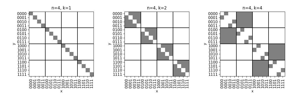
We define a cell on the $i$ th layer of the communication matrix for $\text{\rm NEQ}_{n}^{(k)}$ as a submatrix where the first $i$ parts of the inputs are fixed to some values (see Figure 5). That is, for all $j\leq i$ , $x_{j}=s_{j}$ and $y_{j}=t_{j}$ for some fixed strings $s_{j},t_{j}\in\{0,1\}^{\tfrac{n}{k}}$ . Some cells are monochromatic; more specifically, the cell becomes monochromatic once we fix a block in such a way that $s_{i}\neq t_{i}$ . We call the $i$ th layer of $\text{\rm NEQ}_{n}^{(k)}$ ’s communication matrix 0-dominant if the cells on this layer that are monochromatic cells because of the equality in the $i$ th block of input are 0-monochromatic (this is the case of odd $i$ ). We define 1-dominant layers similarly (they correspond to even $i$ ). The intuition for Lemma 34, Theorem 36, and Theorem 37 is that $\text{\rm NEQ}^{(k)}_{n}$ can be computed more efficiently when 0-dominant layers in its communication matrix “align” with 0-layers of queries in the decision list.

Figure 5: Cell structure of

\text{\rm NEQ}_{n}^{(k)}

function: bigger cell

\text{\rm NEQ}_{n}^{(i+2)}

consists of smaller cells

\overline{\text{\rm NEQ}_{n}^{(i+1)}}

(zeroes off the diagonal indicate that this is the case of odd

i

), which in turn consist of smaller cells

\text{\rm NEQ}_{n}^{(i)}

shown in the middle.

Proof of the following upper bound can be found in the full version of our paper [28].

Lemma 34.

$\text{\rm NEQ}_{n}^{(k)}$ is computable by a $\text{\rm Rect}\text{\rm-DL}_{k,0}$ , $\widehat{\text{\rm LDL}}_{k,0}$ , and an $\text{\rm LDL}_{k,0}$ each of length $2n$ .

Next we prove the key lemma for the lower bound for $\text{\rm NEQ}_{n}^{(k)}$ .

Lemma 35.

Fix a depth $k$ , and suppose $\text{\rm NEQ}_{n}^{(k)}$ is computable by an $\text{\rm LDL}_{k,1}$ $\mathcal{L}$ of size $<2^{n/k}$ . Then for all $i$ , there exists a non-monochromatic cell on layer $i$ in the communication matrix $\text{\rm NEQ}_{n}^{(k)}$ such that none of its entries have been covered by $\mathcal{L}$ ’s queries of depth at most $i$ .

Proof.

We use induction on $i$ . In the base case, where $i=0$ , the claim trivially holds as $\mathcal{L}$ restricted to queries of depth at most zero is simply an empty LDL.

For the inductive step, we suppose the statement holds for $i-1$ ; we show that it is true for $i$ as well. Without loss of generality, let $i$ be odd. Then the $i$ th layer of the communication matrix for $\text{\rm NEQ}_{n}^{(k)}$ is 0-dominant. Since $\mathcal{L}$ is a $\text{\rm LDL}_{k,1}$ , the $i$ th depth layer of $\mathcal{L}$ is a 1-layer. Since the size of $\mathcal{L}$ is $<2^{n/k}$ , there are at most $2^{n/k}-1$ queries in this depth layer; let $q$ be any such query. Since this a 1-layer in $\mathcal{L}$ , the output for $q$ is 1.

Let $C_{i-1}$ be the cell guaranteed by the induction hypothesis. Let the cell $C_{s,i}$ be the set of inputs such that for all $j<i$ , $x_{j}=y_{j}$ are fixed the same way as in $C_{i-1}$ and $x_{i}=y_{i}=s$ . We claim that as in the previous proof each query on this layer intersects at most one of the $C_{s,i}$ cells. Suppose, for the sake of contradiction, that a query $L_{j}(x,y)\leq t_{j}$ is true on inputs $(X,Y)\in C_{s,i}$ and $(X^{\prime}Y^{\prime})\in C_{s^{\prime},i}$ where $(X,Y)$ and $(X^{\prime},Y^{\prime})$ are 1-inputs to $\text{\rm NEQ}_{n}^{(k)}$ . This implies that $x_{i}=y_{i}=s$ , and $x^{\prime}_{i}=y^{\prime}_{i}=s^{\prime}$ . But then if we consider the input $(X,Y^{\prime})$ , we have that $x_{i}=s\neq s^{\prime}=y^{\prime}_{i}$ , and hence, by definition of $\text{\rm NEQ}^{(i-1)}_{n}$ , $(X,Y^{\prime})$ is a 0-input. Identical reasoning shows that $(X^{\prime},Y)$ is a 0-input. Since $(X,Y)$ and $(X^{\prime},Y^{\prime})$ are both 1-inputs, we have that $L_{j}(X,Y)\leq t_{j}$ and $L_{j}(X^{\prime},Y^{\prime})\leq t_{j}$ . However, note that

L_{j}(X^{\prime},Y)+L_{j}(X,Y^{\prime})=L_{j}(X,Y)+L_{j}(X^{\prime},Y^{\prime}% )\leq 2t_{j}.

Thus, there must exist at least one $z\in\{(X^{\prime},Y),(X,Y^{\prime})\}$ such that $L_{j}(z)\leq t_{j}$ , which means that the query $L_{j}(z)\leq t_{j}$ outputs 1. But, since $\{(X^{\prime},Y),(X,Y^{\prime})\}$ are 0-inputs to $\text{\rm NEQ}_{n}^{(k)}$ , this means that $\mathcal{L}$ outputs the incorrect value on $z$ , a contradiction. Hence, each query on this layer intersects at most one of the $C_{s,i}$ . Since this depth layer contains at most $2^{n/k}-1$ queries and there are $2^{n/k}$ cells $C_{s,i}$ , one of these cells must be uncovered, as desired. $\hfill\blacktriangleleft$

Theorem 36.

The size of any $\text{\rm LDL}_{k,1}$ computing $\text{\rm NEQ}_{n}^{(k)}$ has length at least $2^{n/k}$ .

Proof.

Suppose $\text{\rm NEQ}_{n}^{(k)}$ is computable by a $\text{\rm LDL}_{k,1}$ $\mathcal{L}$ of size $<2^{n/k}$ . Then, by Lemma 35, there exists a cell $C$ in layer $k$ (this cell has just one entry) of the communication matrix $\text{\rm NEQ}_{n}^{(k)}$ which has not been covered. Since $\mathcal{L}$ is a $\text{\rm LDL}_{k,1}$ , the $i$ th depth layer of $\mathcal{L}$ is a 1-layer if and only if $i$ is a 0-dominant layer in the communication matrix for $\text{\rm NEQ}_{n}^{(k)}$ , so $\mathcal{L}$ will output the incorrect value on $C$ . $\hfill\blacktriangleleft$

By a very similar argument, we can prove the same lower bound for rectangle decision lists (see proof in our full paper [28]).

Theorem 37.

The size of any $\text{\rm Rect}\text{\rm-DL}_{k,1}$ computing $\text{\rm NEQ}_{n}^{(k)}$ is at least $2^{n/k}$ .

We note that an analogous result for $k$ -Layer Intersection function (see Definition 43 below) follows from the combination of the results of [27] and [14] going through communication complexity.

$\blacktriangleright$ Remark 38.

Note that similar arguments show that the negation $\neg\text{\rm NEQ}_{n}^{(k)}\in\widehat{\text{\rm LDL}}_{k,1}$ , $\neg\text{\rm NEQ}_{n}^{(k)}\in\text{\rm Rect}\text{\rm-DL}_{k,1}$ , and $\neg\text{\rm NEQ}_{n}^{(k)}\notin\text{\rm LDL}_{k,0},\text{\rm Rect}\text{% \rm-DL}_{k,0}$ .

5 ELDL lower bounds

We start by showing that small discrepancy over the uniform distribution implies a bound on depth of ELDLs.

In this argument it will be convenient to work with the notion of advantage of a Boolean function $f$ on a subset $S$ of its inputs:

\operatorname{Adv}(S,f)\mathrel{\mathchoice{\vbox{\hbox{$\displaystyle:$}}}{% \vbox{\hbox{$\textstyle:$}}}{\vbox{\hbox{$\scriptstyle:$}}}{\vbox{\hbox{$% \scriptscriptstyle:$}}}{=}}\Big|\ \left|\{(x,y)\in S\mid f(x,y)=1\}\right|-% \left|\{(x,y)\in S|f(x,y)=0\}\right|\ \Big|.

Advantage is closely related to discrepancy over the uniform distribution in the following way: for any combinatorial rectangle $R$ , we have $\operatorname{Adv}(R,f)=2^{2n}\mathsf{Disc}_{U}(R,f)$ .

We make use of the following lemma, whose proof can be found in the full version of our paper [28].

Lemma 39.

Let $f:\{0,1\}^{n}\times\{0,1\}^{n}\rightarrow\{0,1\}$ be a function such that $\mathsf{Disc}_{U}(f)\leq d$ , where $U$ is the uniform distribution. Then $f$ has advantage of at most $2^{2n+1}\sqrt{d}$ on any blocky system of rectangles.

Theorem 40.

Let $f\colon\{0,1\}^{n}\times\{0,1\}^{n}\to\{0,1\}$ and $\mathsf{Disc}_{U}(f)\leq d$ , where $U$ is the uniform distribution on inputs. Assume that $f$ is approximately balanced; specifically, $|f^{-1}(0)|,|f^{-1}(1)|\geq\Omega(2^{2n})$ . Then the size of any ELDL of depth $k$ computing $f$ is at least $\Omega(kd^{-1/2k})$ .

Proof.

Consider an ELDL of size $s$ and depth $k$ computing $f$ . Denote the number of queries on each layer by $s_{1},\ldots,s_{k}$ . We have $s_{1}+\ldots+s_{k}=s$ .

We prove the following statement by induction on the number of layers. Consider queries on layer $i$ ; assume that they output $b\in\{0,1\}$ . We will prove that these queries together cover at most $2^{2n+i}\sqrt{d}\prod_{j=1}^{i}s_{j}$ entries in $f^{-1}(b)$ .

For the base case, consider the first layer, and denote its output by $b$ . By Lemma 13, a query on this layer defines a blocky matrix. Since $\mathsf{Disc}_{U}(f)\leq d$ , by Lemma 39 this blocky matrix has advantage at most $2^{2n+1}\sqrt{d}$ . Since there are no previous layers, the query cannot cover any inputs $(x,y)$ with $f(x,y)=\neg b$ . Thus, the blocky matrix is monochromatic and covers at most $2^{2n+1}\sqrt{d}$ $b$ -outputs. There are at most $s_{1}$ queries on the first layer, and together they cover at most $2^{2n+1}\sqrt{d}s_{1}$ $b$ -outputs.

For the induction step, assume that the statement is true for all layers before the $i$ th layer. Denote the output of this layer by $b$ and consider a query on the $i$ th layer. The corresponding blocky matrix does not have to be monochromatic since it can contain $\neg b$ -entries covered on the previous layers. The number of $\neg b$ -entries covered on the previous layers is upper bounded by

	$\displaystyle 2^{2n+i-1}\sqrt{d}\prod^{i-1}_{j=1}s_{j}+2^{2n+i-3}\sqrt{d}\prod% ^{i-3}_{j=1}s_{j}+2^{2n+i-5}\sqrt{d}\prod^{i-5}_{j=1}s_{j}+\cdots$	$\displaystyle\leq$
	$\displaystyle\left(2^{i-1}+2^{i-3}+2^{i-5}+\cdots\right)2^{2n}\sqrt{d}\prod^{i% -1}_{j=1}s_{j}$	$\displaystyle\leq(2^{i}-2)2^{2n}\sqrt{d}\prod^{i-1}_{j=1}s_{j}$

for all $i\geq 2$ . By Lemma 39, the number of $b$ -entries covered by this blocky matrix is greater by at most $2^{2n+1}\sqrt{d}$ . Then we get the following upper bound on the number of $b$ -entries covered by this blocky matrix:

2^{2n+i}\sqrt{d}\prod^{i-1}_{j=1}s_{j}.

Since there are at most $s_{i}$ queries on the $i$ th layer, together they cover at most $2^{2n+i}\sqrt{d}\prod^{i}_{j=1}s_{j}$ $b$ -entries, as needed.

Now, assume that the last layer outputs $b$ . Then the number of inputs on which the decision list outputs $b$ is at most

2^{2n+k}\sqrt{d}\prod^{k}_{j=1}s_{j}+2^{2n+k-2}\sqrt{d}\prod^{k-2}_{j=1}s_{j}+% 2^{2n+k-4}\sqrt{d}\prod^{k-4}_{j=1}s_{j}+\cdots\leq 2^{2n+k+1}\sqrt{d}\prod^{k% }_{j=1}s_{j}.

Since the function is approximately balanced, we have that

2^{2n+k+1}\sqrt{d}\prod^{k}_{j=1}s_{j}\geq\Omega(2^{2n})

using the AM-GM inequality and observing that $s_{1}+\ldots+s_{k}=s$ gives the bound

s\geq\Omega(kd^{-1/2k}).\

$\hfill\blacktriangleleft$

Since $\mathsf{Disc}_{U}(\text{\rm IP}_{n})=2^{-n/2}$ [21] we immediately get the following corollary.

Corollary 41.

The size of an ELDL of depth $k$ computing the Inner-Product function $\text{\rm IP}_{n}$ is at least $k2^{\Omega(n/k)}$ .

$\blacktriangleright$ Remark 42.

Observe that since $2^{\Theta(n/k)}\geq\Theta(n/k)$ , Corollary 41 gives a linear lower bound on the size of ELDL for IP. However, note that this bound on the size also follows from the standard argument based on the size of rectangles. For this, one can consider the first query and consider a square submatrix of the communication matrix of size roughly $2^{n}/2\times 2^{n}/2$ such that the first query does not produce an output on this rectangle. Then one can argue by induction. This approach is very similar to the approach in [3].

Next we proceed to showing that ELDLs of fixed depth form a hierarchy. The separating functions in this case are $\text{\rm INT}_{n}^{(k)}$ , which we define below:

Definition 43 ( $k$ -Layer Intersection).

For a positive integer $n$ , the $k$ -Layer Intersection function on $2n$ inputs, denoted $\text{\rm INT}_{n}^{(k)}$ (see Figure 6 below), is the composition $\text{\rm EMB}_{k}\circ\text{\rm INT}_{n/k}$ is defined by

\text{\rm INT}_{n}^{(k)}(x_{1},y_{1},\ldots,x_{k},y_{k})=1\iff\min\{i\in[n]% \mid x_{i}\cap y_{i}\neq\emptyset\}\text{\emph{ is even.}}

Similar to $\text{\rm NEQ}_{n}^{(k)}$ and EMB (see Definition 18), we say that $\text{\rm INT}_{n}^{(k)}(x_{1},y_{1},\ldots,x_{k},y_{k})=0$ in the case that $x_{i}\cap y_{i}=\emptyset$ for all $i$ if $k$ is even, and $\text{\rm INT}_{n}^{(k)}(x_{1},y_{1},\ldots,x_{k},y_{k})=1$ in the case that $x_{i}\cap y_{i}=\emptyset$ for all $i$ if $k$ is odd.

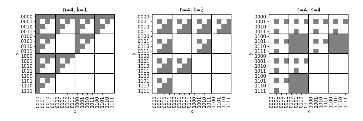
We start with the upper bound, for which the proof can be found in the full version of our paper [28].

Lemma 44.

$\text{\rm INT}_{n}^{(k)}$ is computable by an $\text{\rm ELDL}_{k,0}$ of length $n$ .

We will use the following well-known property of Disjointness (see, e.g., [21] Chapter 1, exercise 1.26).

Claim 45.

Let $M$ be the communication matrix for $\text{\rm DISJ}_{n}$ . Then if $R$ is a 1-monochromatic rectangle in $M$ , $|R|\leq 2^{n}$ .

The rest of the section is devoted to the proof of the following theorem, which gives an exponential lower bound for the size of ELDLs when the depth $k=O(\sqrt{n})$ .

Theorem 46.

Any $\text{\rm ELDL}_{k,1}$ computing $\text{\rm INT}_{n}^{(k)}$ has size $2^{\Omega(n/k)-O(k)}$ .

For the proof of this theorem, it is convenient to change the notation slightly and talk about functions with $2nk$ input variables. That is, we will consider functions $\text{\rm INT}_{nk}^{(k)}$ and the lower bound we will prove is $2^{\Omega(n)-O(k)}$ .

Note that the cells of $\text{\rm INT}_{n}^{(k)}$ have essentially the same structure as the $\text{\rm DISJ}_{n}$ function. It is helpful for this argument to restrict $\text{\rm DISJ}_{n}$ to a submatrix with the same number of ones in each row and column. To do this, we restrict the input to $\text{\rm DISJ}_{n}$ to subsets of size exactly $\tfrac{n}{3}$ . In other words, the inputs to $\text{\rm DISJ}_{n}$ are now restricted to $(X,Y)$ such that $|X|=|Y|=\tfrac{n}{3}$ . The number of $n$ -bit strings satisfying this condition is

\binom{n}{n/3}=2^{H\left(1/3\right)n(1+o(1))},

where $H(x)$ is the binary entropy function. We will denote this number by $N$ . Note also that for a fixed row (column) in the restricted submatrix, the number of ones in it is

\binom{2n/3}{n/3}=2^{\tfrac{2n}{3}(1+o(1))}.

We will denote this number by $D$ . By Claim 45, the size of the largest $1$ -monochromatic rectangle is still at most $2^{n}$ .

We propagate this restriction to $\text{\rm INT}_{nk}^{(k)}$ . In other words, we view the input to $\text{\rm INT}_{nk}^{(k)}$ as $((X_{1},Y_{1}),\ldots,(X_{k},Y_{k}))$ , where each $X_{i},Y_{i}\in\{0,1\}^{n}$ have $|X_{i}|=|Y_{i}|=\tfrac{n}{3}$ . In particular, the number of rows and columns in $\text{\rm INT}_{nk}^{(k)}$ is $N^{k}$ . Hereafter, in this section, when we refer to $\text{\rm INT}_{nk}^{(k)}$ or $\text{\rm DISJ}_{n}$ , we actually mean these restricted versions.

We start by establishing some useful properties of the $\text{\rm DISJ}_{n}$ function. A proof of the following lemma is in the full version of our paper [28].

Lemma 47.

Let $N$ and $D$ be defined as above. If we arbitrarily remove at most $N/10$ rows and at most $N/10$ columns from the communication matrix of $\text{\rm DISJ}_{n}$ , the number of ones in the resulting matrix is at least $4ND/5$ .

Moreover, there exists a set of additional rows and a set of additional columns such that on their removal we obtain a matrix with at least $N/2$ rows and at least $N/2$ columns such that any row and any column contains at least $3D/8$ ones.

Analogously to the case of $\text{\rm NEQ}_{n}^{(k)}$ , we define a cell on the $i$ th layer of $\text{\rm INT}_{nk}^{(k)}$ to be a submatrix where the first $i$ parts of the inputs are fixed to some values. That is, $x_{j}=s_{j}$ and $y_{j}=t_{j}$ for some fixed strings $s_{j},t_{j}\in\{0,1\}^{n}$ for all $j\leq i$ . Some cells are monochromatic; more specifically the cell is monochromatic if one of its blocks is fixed in a way that $X_{i}\cap Y_{i}\neq\emptyset$ . We call a layer $i$ of $\text{\rm INT}_{nk}^{(k)}$ 0-dominant if the cells on $i$ th layer that are monochromatic because of the intersection in the $i$ th block are 0-monochromatic. We define 1-dominant layers similarly. In particular, the first layer is $0$ -dominant for $\text{\rm INT}^{k}_{nk}$ . We say that a row or column of a cell is covered by a rectangle $R$ if it has non-empty intersection with $R$ . When it is clear from context, we will refer to a column as covered if one of the rectangles we are currently considering intersects it.

Next, we state the key lemma needed for the proof of Theorem 46. As in Section 4, the intuition behind the result is that it is hard to compute $\text{\rm INT}_{nk}^{(k)}$ when $0$ -dominant layers of the communication matrix do not align with 0-layers of queries in the decision list.

Lemma 48.

Fix a depth $k$ , and suppose $\text{\rm INT}_{nk}^{(k)}$ is computable by an $\text{\rm ELDL}_{k,1}$ $\mathcal{E}$ of size $S$ . Define $\varepsilon_{0}=0$ and $\varepsilon_{i}=11^{i}\cdot\frac{8}{3}\cdot\frac{2^{n/2}S}{D}$ for all $1\leq i\leq k$ . Then for all $i$ , there exists a non-monochromatic cell on layer $i$ in $\text{\rm INT}_{nk}^{(k)}$ such that $\leq\varepsilon_{i}$ fraction of its rows and columns have been covered by $\mathcal{E}$ ’s queries of depth at most $i$ .

The proof of Theorem 46 based on the Lemma 48 is analogous to the proofs from Section 4.

Proof of Theorem 46.

Suppose $\text{\rm INT}_{nk}^{(k)}$ is computable by an $\text{\rm ELDL}_{k,1}$ $\mathcal{E}$ of size $S$ . Then, by Lemma 48, there exists a cell on layer $k$ such that at most $\varepsilon_{k}=11^{k}\cdot\frac{8}{3}\cdot\frac{2^{n/2}S}{D}$ fraction of its rows and columns have been covered by $\mathcal{E}$ ’s queries of depth at most $k$ . Note that the cells on $k$ th layer are $1\times 1$ matrices and if $\varepsilon_{k}<1$ , then the only entry of this matrix is not covered, and $\mathcal{E}$ outputs an incorrect value on it (since the ELDL outputs $b$ on $(1-b)$ -dominant layers of the communication matrix). From that, we observe that the decision list is incorrect if

11^{k}\cdot\frac{8}{3}\cdot\frac{2^{n/2}S}{D}<1

and given that $D=2^{\tfrac{2n}{3}(1+o(1))}$ , the theorem follows. $\hfill\blacktriangleleft$

Figure 7: The notion of projection: a rectangle over the iterated matrix translates to a rectangle over the cells in DISJ matrix.

Now it remains only to prove Lemma 48.

Proof of Lemma 48.

We use induction on $i$ . For the base case, we consider $i=0$ . For this case, no parts of the inputs are fixed and thus there is only one cell, the whole matrix. Clearly, an $\varepsilon_{0}=0$ fraction of its rows and columns have been covered by $\mathcal{E}$ ’s queries of depth at most $0$ .

For the induction step, suppose that the statement holds for the $(i-1)$ st layer of $\text{\rm INT}_{nk}^{(k)}$ and consider the corresponding cell $M^{(i-1)}$ on the $(i-1)$ st layer. We show that the statement is true for the $i$ th layer as well. The cell we are going to find is a submatrix of the cell on the $(i-1)$ st layer. Without loss of generality, let the $i$ th layer be a 0-dominant layer. We view the matrix $M^{(i-1)}$ as a block-matrix, in which blocks correspond to cells of the $i$ th layer and each block is either a constant 0 matrix, or an $M^{(i)}$ matrix corresponding to the non-monochromatic cell on the next layer. That is, consider the part of input $(X_{i}$ , $Y_{i})$ corresponding to the $i$ th layer and consider the communication matrix $M_{\text{\rm DISJ}}$ of DISJ on these inputs. This matrix reflects the structure of the cells of layer $i$ in $M^{(i-1)}$ : each cell is labeled by specific values of $(X_{i},Y_{i})$ and the cell is 0-monochromatic if and only if $\text{\rm DISJ}(X_{i},Y_{i})=0$ .

By the induction hypothesis, at most an $\varepsilon_{i-1}$ fraction of the rows and columns of $M^{(i-1)}$ are covered by previous queries. First we remove block-rows and block-columns that have more than $10\varepsilon_{i-1}$ fraction of their rows and columns respectively covered. By Markov’s inequality, this way we remove at most $1/10$ fraction of all block-rows and block-columns. In the remaining block-rows and block-columns we further remove rows and columns that are covered. In each block we remove at most $10\varepsilon_{i-1}$ fraction of rows and columns.

As we observed, the block-matrix has the same structure as the Disjointness function. By Lemma 47 we can further remove constant fraction of block-rows and block-columns in such a way that the number of block-rows and block-columns is still at least $N/2$ and each of the remaining block-rows and block-columns contains at least $3D/8$ non-monochromatic cells. For notation convenience, denote the resulting submatrix by $M^{(i-1)}$ again.

Now consider queries of the $i$ th depth layer of $\mathcal{E}$ . Since the size of $\mathcal{E}$ is $S$ , there are at most $S$ queries in this layer. Since $\mathcal{E}$ is an ELDL, each of its queries can be expressed as a blocky system of rectangles. Consider some query on the $i$ th layer, and let $M$ denote the corresponding blocky system within $M^{(i-1)}$ . Let $R_{1},\ldots R_{t}$ with $R_{j}=A_{j}\times B_{j}$ be rectangles in $M$ . Note that since we removed all rows and columns partially covered by the queries of the previous layer, these rectangles must be 1-monochromatic. We want to show that the $R_{j}$ s cannot cover too much of the matrix $M^{(i-1)}$ . For each rectangle $R_{j}$ , consider its projection $R_{j}^{\prime}=A_{j}^{\prime}\times B_{j}^{\prime}$ to inputs $(X_{i},Y_{i})$ (see Figure 7). That is, if $R_{j}$ contains an entry with some specific values of $(X_{i},Y_{i})$ , then these values of $(X_{i},Y_{i})$ are in $R_{j}^{\prime}$ . Basically, $R_{j}^{\prime}$ represents the rectangle of cells in $M_{\text{\rm DISJ}}$ that are intersecting with $R_{j}$ . Note that since $R_{j}$ is 1-monochromatic, it cannot intersect 0-cells, and thus $R_{j}^{\prime}$ is a 1-monochromatic rectangle in $M_{\text{\rm DISJ}}$ .

Note that we can decompose $M$ into two disjoint matrices $M_{wide}$ and $M_{tall}$ based on the dimensions of the rectangles $R_{j}^{\prime}$ . In particular, the rectangle $R_{j}=A_{j}\times B_{j}$ is in $M_{wide}$ if $|A_{j}^{\prime}|<2^{\frac{n}{2}}$ and in $M_{tall}$ if $|B_{j}^{\prime}|<2^{\frac{n}{2}}$ . Intuitively, $M_{wide}$ contains all rectangles that are short and $M_{tall}$ contains all rectangles that are narrow. Note that by Claim 45 each rectangle is either short or narrow.

We will argue that $M_{wide}$ has small intersection with a random non-monochromatic cell in $M^{(i-1)}$ . A symmetric argument shows that it is also true for $M_{tall}$ , and hence for $M$ .

Fix some column of cells $c_{l}$ in $M^{(i-1)}$ . We make use of the following claim:

Claim 49.

We have $|B_{1}\cap c_{l}|+\cdots+|B_{t}\cap c_{l}|\leq W,$ where $W$ is the number of columns in $c_{l}$ .

Indeed, the claim holds since $M_{wide}$ is blocky and therefore distinct rectangles do not overlap in columns.

Pick a uniformly random multicolored cell $C$ in $c_{l}$ . Let $X$ be a random variable for the fraction of $C$ ’s columns which have a non-empty intersection with one of the rectangles $R_{j}\in M_{wide}$ . We have the following upper bound on the expected number of covered columns in a non-monochromatic cell $C$ :

\mathbb{E}_{C\sim c_{l}}[X]\leq\sum_{j=1}^{t}\frac{|B_{j}\cap c_{l}|}{W}\cdot% \frac{A_{j}^{\prime}}{\frac{3D}{8}}\leq\frac{1}{W}\sum_{j=1}^{t}|B_{j}\cap c_{% l}|\cdot\frac{2^{\frac{n}{2}}}{\frac{3D}{8}}\leq\frac{W\cdot 2^{\frac{n}{2}}}{% W\cdot\frac{3D}{8}}=\frac{2^{\frac{n}{2}}}{\frac{3D}{8}}.

(1)

Let $X^{r}$ be the random variable denoting the fraction of columns covered by $M_{wide}$ in a uniformly random non-monochromatic cell $C$ in the matrix $M^{(i-1)}$ . Similarly, let $X^{c}$ be the random variable denoting the fraction of rows covered by $M_{tall}$ in a uniformly random non-monochromatic cell in the matrix.

Since (1) holds for each column of cells $c_{l}$ , we have $\mathbb{E}_{C\sim M^{(i-1)}}[X^{r}]\leq\frac{8}{3}\cdot\frac{2^{n/2}}{D}$ and the same is true for $X^{c}$ . We have this bound for each query on layer $i$ and since there are at most $S$ queries in this layer, the total expected fraction of rows and columns covered for a random cell is bounded by $\frac{8}{3}\cdot\frac{2^{n/2}S}{D}$ . By Markov’s inequality there is a cell on the $i$ th layer that has both at most $10\cdot\frac{8}{3}\cdot\frac{2^{n/2}S}{D}$ fraction of its rows and at most $10\cdot\frac{8}{3}\cdot\frac{2^{n/2}S}{D}$ fraction of its columns covered. Together with rows and columns covered on the previous layers, we have that for this cell at most

10\varepsilon_{i-1}+10\cdot\frac{8}{3}\cdot\frac{2^{n/2}S}{D}\leq 10% \varepsilon_{i-1}+\varepsilon_{i-1}\leq\varepsilon_{i}

rows and columns are covered, as needed. $\hfill\blacktriangleleft$

References

[1] Prashanth Amireddy, Sai Jayasurya, and Jayalal Sarma. Power of decision trees with monotone queries. In Donghyun Kim, R. N. Uma, Zhipeng Cai, and Dong Hoon Lee, editors, Computing and Combinatorics - 26th International Conference, COCOON 2020, Atlanta, GA, USA, August 29-31, 2020, Proceedings, Lecture Notes in Computer Science, pages 287–298. Springer, 2020. doi:10.1007/978-3-030-58150-3_23.
[2] Avrim Blum and Mona Singh. Learning functions of k terms. In Proceedings of the Third Annual Workshop on Computational Learning Theory, COLT ’90, pages 144–153, San Francisco, CA, USA, 1990. Morgan Kaufmann Publishers Inc. URL: http://dl.acm.org/citation.cfm?id=92620.
[3] Arkadev Chattopadhyay, Meena Mahajan, Nikhil S. Mande, and Nitin Saurabh. Lower bounds for linear decision lists. Chic. J. Theor. Comput. Sci., 2020, 2020. URL: http://cjtcs.cs.uchicago.edu/articles/2020/1/contents.html.
[4] Arkadev Chattopadhyay and Nikhil Mande. A short list of equalities induces large sign rank. In 2018 IEEE 59th Annual Symposium on Foundations of Computer Science (FOCS), pages 47–58, 2018. doi:10.1109/FOCS.2018.00014.
[5] Yogesh Dahiya, Vignesh K., Meena Mahajan, and Karteek Sreenivasaiah. Linear threshold functions in decision lists, decision trees, and depth-2 circuits. Information Processing Letters, 183:106418, 2024. doi:10.1016/j.ipl.2023.106418.
[6] Mason DiCicco, Vladimir Podolskii, and Daniel Reichman. Nearest neighbor complexity and boolean circuits. In Raghu Meka, editor, 16th Innovations in Theoretical Computer Science Conference, ITCS 2025, January 7-10, 2025, Columbia University, New York, NY, USA, volume 325 of LIPIcs, pages 42:1–42:23. Schloss Dagstuhl – Leibniz-Zentrum für Informatik, 2025. doi:10.4230/LIPIcs.ITCS.2025.42.
[7] Jürgen Forster. A linear lower bound on the unbounded error probabilistic communication complexity. Journal of Computer and System Sciences, 65(4):612–625, 2002. doi:10.1016/S0022-0000(02)00019-3.
[8] Jürgen Forster, Matthias Krause, Satyanarayana V. Lokam, Rustam Mubarakzjanov, Niels Schmitt, and Hans Ulrich Simon. Relations between communication complexity, linear arrangements, and computational complexity. In FSTTCS, pages 171–182, 2001. doi:10.1007/3-540-45294-X_15.
[9] Mikael Goldmann. Communication Complexity and Lower Bounds for Threshold Circuits, pages 85–125. Springer US, Boston, MA, 1994. doi:10.1007/978-1-4615-2696-4_3.
[10] Mikael Goldmann, Johan Håstad, and Alexander Razborov. Majority gates vs. general weighted threshold gates. Comput. Complex., pages 277–300, 1992. doi:10.1007/BF01200426.
[11] Mika Göös, Pritish Kamath, Toniann Pitassi, and Thomas Watson. Query-to-Communication Lifting for $P^{NP}$ . In Ryan O’Donnell, editor, 32nd Computational Complexity Conference (CCC 2017), volume 79 of Leibniz International Proceedings in Informatics (LIPIcs), pages 12:1–12:16, Dagstuhl, Germany, 2017. Schloss Dagstuhl – Leibniz-Zentrum für Informatik. doi:10.4230/LIPIcs.CCC.2017.12.
[12] Mika Göös, Toniann Pitassi, and Thomas Watson. The landscape of communication complexity classes. Comput. Complex., 27(2):245–304, June 2018. doi:10.1007/S00037-018-0166-6.
[13] András Hajnal, Wolfgang Maass, Pavel Pudlak, Mario Szegedy, and Gyorgy Turan. Threshold circuits of bounded depth. J. Comput. Syst. Sci., 46:129–154, April 1993. doi:10.1109/SFCS.1987.59.
[14] Bernd Halstenberg and Rüdiger Reischuk. Relations between communication complexity classes. J. Comput. Syst. Sci., 41(3):402–429, 1990. doi:10.1016/0022-0000(90)90027-I.
[15] Lianna Hambardzumyan, Hamed Hatami, and Pooya Hatami. Dimension-free bounds and structural results in communication complexity. Isr. J. Math., 253(2):555–616, March 2023.
[16] Kristoffer Arnsfelt Hansen and Vladimir V. Podolskii. Exact threshold circuits. In 2010 IEEE 25th Annual Conference on Computational Complexity, pages 270–279, 2010. doi:10.1109/CCC.2010.33.
[17] Kristoffer Arnsfelt Hansen and Vladimir V. Podolskii. Polynomial threshold functions and boolean threshold circuits. Information and Computation, 240:56–73, 2015. MFCS 2013. doi:10.1016/j.ic.2014.09.008.
[18] Russell Impagliazzo and Ryan Williams. Communication complexity with synchronized clocks. In 2010 IEEE 25th Annual Conference on Computational Complexity, pages 259–269, 2010. doi:10.1109/CCC.2010.32.
[19] Stasys Jukna. Extremal Combinatorics - With Applications in Computer Science. Texts in Theoretical Computer Science. An EATCS Series. Springer, 2011. doi:10.1007/978-3-642-17364-6.
[20] Stasys Jukna et al. Boolean function complexity: advances and frontiers, volume 27. Springer, 2012. doi:10.1007/978-3-642-24508-4.
[21] Eyal Kushilevitz and Noam Nisan. Communication complexity. Cambridge University Press, 1997.
[22] M. Minsky and S. Papert. Perceptrons; an Introduction to Computational Geometry. MIT Press, 1969. URL: https://books.google.com/books?id=Ow1OAQAAIAAJ.
[23] J Myhill and W H Kautz. On the size of weights required for linear-input switching functions. IEEE Trans. Electron. Comput., EC-10(2):288–290, June 1961. doi:10.1109/TEC.1961.5219204.
[24] Ziv Nevo and Ran El-Yaniv. On online learning of decision lists. The Journal of Machine Learning Research, 3:271–301, September 2002. doi:10.1162/153244303765208395.
[25] Periklis Papakonstantinou, Dominik Scheder, and Hao Song. Overlays and limited memory communication. In 2014 IEEE 29th Conference on Computational Complexity (CCC), pages 298–308, 2014. doi:10.1109/CCC.2014.37.
[26] Ramamohan Paturi and Janos Simon. Probabilistic communication complexity. Journal of Computer and System Sciences, 33(1):106–123, 1986. doi:10.1016/0022-0000(86)90046-2.
[27] Toniann Pitassi, Morgan Shirley, and Thomas Watson. Nondeterministic and randomized boolean hierarchies in communication complexity. Comput. Complex., 30(2):10, 2021. doi:10.1007/S00037-021-00210-5.
[28] Vladimir Podolskii and Morgan E. Prior. Alternation depth of threshold decision lists. Electron. Colloquium Comput. Complex., TR25, 2025. URL: https://eccc.weizmann.ac.il/report/2025/143.
[29] Anup Rao and Amir Yehudayoff. Communication complexity: and applications. Cambridge University Press, 2020.
[30] Alexander A Razborov. On small depth threshold circuits. In Scandinavian Workshop on Algorithm Theory, pages 42–52. Springer, 1992. doi:10.1007/3-540-55706-7_4.
[31] Alexander A Razborov and Alexander A Sherstov. The sign-rank of AC⁰. SIAM Journal on Computing, 39(5):1833–1855, 2010.
[32] György Turán and Farrokh Vatan. Linear decision lists and partitioning algorithms for the construction of neural networks. In Felipe Cucker and Michael Shub, editors, Foundations of Computational Mathematics, pages 414–423, Berlin, Heidelberg, 1997. Springer Berlin Heidelberg.

[bib.bib1] [1] Prashanth Amireddy, Sai Jayasurya, and Jayalal Sarma. Power of decision trees with monotone queries. In Donghyun Kim, R. N. Uma, Zhipeng Cai, and Dong Hoon Lee, editors, Computing and Combinatorics - 26th International Conference, COCOON 2020, Atlanta, GA, USA, August 29-31, 2020, Proceedings, Lecture Notes in Computer Science, pages 287–298. Springer, 2020. doi:10.1007/978-3-030-58150-3_23.

[bib.bib2] [2] Avrim Blum and Mona Singh. Learning functions of k terms. In Proceedings of the Third Annual Workshop on Computational Learning Theory, COLT ’90, pages 144–153, San Francisco, CA, USA, 1990. Morgan Kaufmann Publishers Inc. URL: http://dl.acm.org/citation.cfm?id=92620.

[bib.bib3] [3] Arkadev Chattopadhyay, Meena Mahajan, Nikhil S. Mande, and Nitin Saurabh. Lower bounds for linear decision lists. Chic. J. Theor. Comput. Sci., 2020, 2020. URL: http://cjtcs.cs.uchicago.edu/articles/2020/1/contents.html.

[bib.bib4] [4] Arkadev Chattopadhyay and Nikhil Mande. A short list of equalities induces large sign rank. In 2018 IEEE 59th Annual Symposium on Foundations of Computer Science (FOCS), pages 47–58, 2018. doi:10.1109/FOCS.2018.00014.

[bib.bib5] [5] Yogesh Dahiya, Vignesh K., Meena Mahajan, and Karteek Sreenivasaiah. Linear threshold functions in decision lists, decision trees, and depth-2 circuits. Information Processing Letters, 183:106418, 2024. doi:10.1016/j.ipl.2023.106418.

[bib.bib6] [6] Mason DiCicco, Vladimir Podolskii, and Daniel Reichman. Nearest neighbor complexity and boolean circuits. In Raghu Meka, editor, 16th Innovations in Theoretical Computer Science Conference, ITCS 2025, January 7-10, 2025, Columbia University, New York, NY, USA, volume 325 of LIPIcs, pages 42:1–42:23. Schloss Dagstuhl – Leibniz-Zentrum für Informatik, 2025. doi:10.4230/LIPIcs.ITCS.2025.42.

[bib.bib7] [7] Jürgen Forster. A linear lower bound on the unbounded error probabilistic communication complexity. Journal of Computer and System Sciences, 65(4):612–625, 2002. doi:10.1016/S0022-0000(02)00019-3.

[bib.bib8] [8] Jürgen Forster, Matthias Krause, Satyanarayana V. Lokam, Rustam Mubarakzjanov, Niels Schmitt, and Hans Ulrich Simon. Relations between communication complexity, linear arrangements, and computational complexity. In FSTTCS, pages 171–182, 2001. doi:10.1007/3-540-45294-X_15.

[bib.bib9] [9] Mikael Goldmann. Communication Complexity and Lower Bounds for Threshold Circuits, pages 85–125. Springer US, Boston, MA, 1994. doi:10.1007/978-1-4615-2696-4_3.

[bib.bib10] [10] Mikael Goldmann, Johan Håstad, and Alexander Razborov. Majority gates vs. general weighted threshold gates. Comput. Complex., pages 277–300, 1992. doi:10.1007/BF01200426.

[bib.bib11] [11] Mika Göös, Pritish Kamath, Toniann Pitassi, and Thomas Watson. Query-to-Communication Lifting for $P^{NP}$ . In Ryan O’Donnell, editor, 32nd Computational Complexity Conference (CCC 2017), volume 79 of Leibniz International Proceedings in Informatics (LIPIcs), pages 12:1–12:16, Dagstuhl, Germany, 2017. Schloss Dagstuhl – Leibniz-Zentrum für Informatik. doi:10.4230/LIPIcs.CCC.2017.12.

[bib.bib12] [12] Mika Göös, Toniann Pitassi, and Thomas Watson. The landscape of communication complexity classes. Comput. Complex., 27(2):245–304, June 2018. doi:10.1007/S00037-018-0166-6.

[bib.bib13] [13] András Hajnal, Wolfgang Maass, Pavel Pudlak, Mario Szegedy, and Gyorgy Turan. Threshold circuits of bounded depth. J. Comput. Syst. Sci., 46:129–154, April 1993. doi:10.1109/SFCS.1987.59.

[bib.bib14] [14] Bernd Halstenberg and Rüdiger Reischuk. Relations between communication complexity classes. J. Comput. Syst. Sci., 41(3):402–429, 1990. doi:10.1016/0022-0000(90)90027-I.

[bib.bib15] [15] Lianna Hambardzumyan, Hamed Hatami, and Pooya Hatami. Dimension-free bounds and structural results in communication complexity. Isr. J. Math., 253(2):555–616, March 2023.

[bib.bib16] [16] Kristoffer Arnsfelt Hansen and Vladimir V. Podolskii. Exact threshold circuits. In 2010 IEEE 25th Annual Conference on Computational Complexity, pages 270–279, 2010. doi:10.1109/CCC.2010.33.

[bib.bib17] [17] Kristoffer Arnsfelt Hansen and Vladimir V. Podolskii. Polynomial threshold functions and boolean threshold circuits. Information and Computation, 240:56–73, 2015. MFCS 2013. doi:10.1016/j.ic.2014.09.008.

[bib.bib18] [18] Russell Impagliazzo and Ryan Williams. Communication complexity with synchronized clocks. In 2010 IEEE 25th Annual Conference on Computational Complexity, pages 259–269, 2010. doi:10.1109/CCC.2010.32.

[bib.bib19] [19] Stasys Jukna. Extremal Combinatorics - With Applications in Computer Science. Texts in Theoretical Computer Science. An EATCS Series. Springer, 2011. doi:10.1007/978-3-642-17364-6.

[bib.bib20] [20] Stasys Jukna et al. Boolean function complexity: advances and frontiers, volume 27. Springer, 2012. doi:10.1007/978-3-642-24508-4.

[bib.bib21] [21] Eyal Kushilevitz and Noam Nisan. Communication complexity. Cambridge University Press, 1997.

[bib.bib22] [22] M. Minsky and S. Papert. Perceptrons; an Introduction to Computational Geometry. MIT Press, 1969. URL: https://books.google.com/books?id=Ow1OAQAAIAAJ.

[bib.bib23] [23] J Myhill and W H Kautz. On the size of weights required for linear-input switching functions. IEEE Trans. Electron. Comput., EC-10(2):288–290, June 1961. doi:10.1109/TEC.1961.5219204.

[bib.bib24] [24] Ziv Nevo and Ran El-Yaniv. On online learning of decision lists. The Journal of Machine Learning Research, 3:271–301, September 2002. doi:10.1162/153244303765208395.

[bib.bib25] [25] Periklis Papakonstantinou, Dominik Scheder, and Hao Song. Overlays and limited memory communication. In 2014 IEEE 29th Conference on Computational Complexity (CCC), pages 298–308, 2014. doi:10.1109/CCC.2014.37.

[bib.bib26] [26] Ramamohan Paturi and Janos Simon. Probabilistic communication complexity. Journal of Computer and System Sciences, 33(1):106–123, 1986. doi:10.1016/0022-0000(86)90046-2.

[bib.bib27] [27] Toniann Pitassi, Morgan Shirley, and Thomas Watson. Nondeterministic and randomized boolean hierarchies in communication complexity. Comput. Complex., 30(2):10, 2021. doi:10.1007/S00037-021-00210-5.

[bib.bib28] [28] Vladimir Podolskii and Morgan E. Prior. Alternation depth of threshold decision lists. Electron. Colloquium Comput. Complex., TR25, 2025. URL: https://eccc.weizmann.ac.il/report/2025/143.

[bib.bib29] [29] Anup Rao and Amir Yehudayoff. Communication complexity: and applications. Cambridge University Press, 2020.

[bib.bib30] [30] Alexander A Razborov. On small depth threshold circuits. In Scandinavian Workshop on Algorithm Theory, pages 42–52. Springer, 1992. doi:10.1007/3-540-55706-7_4.

[bib.bib31] [31] Alexander A Razborov and Alexander A Sherstov. The sign-rank of AC⁰. SIAM Journal on Computing, 39(5):1833–1855, 2010.

[bib.bib32] [32] György Turán and Farrokh Vatan. Linear decision lists and partitioning algorithms for the construction of neural networks. In Felipe Cucker and Michael Shub, editors, Foundations of Computational Mathematics, pages 414–423, Berlin, Heidelberg, 1997. Springer Berlin Heidelberg.

Alternation Depth of Threshold Decision Lists

Abstract

Keywords and phrases:

Category:

Copyright and License:

2012 ACM Subject Classification:

Related Version:

Acknowledgements:

DOI:

Event:

Editors:

Series and Publisher:

1 Introduction

Our results

Theorem (informal version of Theorem 29).

Theorem (informal version of Theorem 31).

Theorem (informal version of Theorem 36).

Theorem (informal version of Corollary 41).

Theorem (informal version of Theorem 46).

2 Preliminaries

2.1 Communication Complexity

Definition 1 (Communication matrix).

Definition 2 (Combinatorial rectangle).

Definition 3 (Monochromatic combinatorial rectangle).

Definition 4 (Function class Rect).

Definition 5 (Discrepancy).

2.2 Complexity Classes

Definition 6 (LTF, LTF^).

Definition 7 (ELTF).

Definition 8 (S-decision list, LDL, LDL^, ELDL, Rect-DL, DL).

▶ Remark 9.

Lemma 10.

Definition 11 (Blocky system of rectangles).

Definition 12 (Blocky matrix).

Lemma 13.

Definition 14 (Alternation depth).

▶ Remark 15.

Definition 16 (PNPc⁢c [12]).

2.3 Relevant Functions

Definition 17.

Definition 18 (Even-Min-Bit).

3 Initial Observations

Proposition 19.

Proposition 20.

Lemma 21.

Proposition 22.

Proposition 23.

Proposition 24.

Proposition 25.

Proposition 26.

Lemma 27.

4 Bounds for LDL and Rect-DL

Lemma 28.

Theorem 29.

Proof.

Lemma 30.

Theorem 31.

Proof of Theorem 31.

Corollary 32.

Definition 33 (k-Layer Non-Equality).

Lemma 34.

Lemma 35.

Proof.

Theorem 36.

Proof.

Theorem 37.

▶ Remark 38.

5 ELDL lower bounds

Lemma 39.

Theorem 40.

Proof.

Corollary 41.

▶ Remark 42.

Definition 43 (k-Layer Intersection).

Lemma 44.

Claim 45.

Theorem 46.

Lemma 47.

Lemma 48.

Proof of Theorem 46.

Definition 6 (LTF, $\widehat{\text{\rm LTF}}$ ).

Definition 8 ( $S$ -decision list, LDL, $\widehat{\text{\rm LDL}}$ , ELDL, Rect-DL, DL).

$\blacktriangleright$ Remark 9.

$\blacktriangleright$ Remark 15.

Definition 16 ( $\text{\rm P}^{\text{\rm NP}^{cc}}$ [12]).

Definition 33 ( $k$ -Layer Non-Equality).

$\blacktriangleright$ Remark 38.

$\blacktriangleright$ Remark 42.

Definition 43 ( $k$ -Layer Intersection).