Dynamic Set Cover with Worst-Case Recourse

Solomon, Shay; Uzrad, Amitai

doi:10.4230/LIPIcs.ICALP.2026.153

Dynamic Set Cover with Worst-Case Recourse

Shay Solomon

Tel Aviv University, Israel Amitai Uzrad

Tel Aviv University, Israel

Abstract

In the dynamic set cover (SC) problem, the input is a dynamic universe of at most $n$ elements and a fixed collection of $m$ sets, where each element belongs to at most $f$ sets and each set has a cost in $[1/C,1]$ . The objective is to efficiently maintain an approximate minimum SC under element updates. Efficiency is primarily measured by the update time, but another important parameter is the recourse (the number of changes to solution per update). Ideally, one would like to achieve low worst-case bounds on both update time and recourse.

One can achieve an approximation of $(1+\epsilon)\ln n$ (greedy-based) or $(1+\epsilon)f$ (primal–dual-based) with worst-case update time $O(f\log n)$ (ignoring $\epsilon$ -dependencies). However, despite a large body of work, no algorithm with low update time (even amortized) and nontrivial worst-case recourse is known even for unweighted instances ( $C=1$ )!

We remedy this by providing a transformation that, given a SC algorithm with approximation $\alpha$ and update time $T$ as a black-box, returns a set cover algorithm with approximation $(2+\epsilon)\alpha$ , update time $O(T+\alpha C)$ and worst-case recourse $O(\alpha C)$ . Our main results are obtained by leveraging this transformation for constant $C$ :

$\blacksquare$

For $f=O(\log n)$ , applying the transformation on the best primal-dual-based algorithm yields worst-case recourse $O(f)$ . For constant $f$ (e.g., vertex cover), we get near-optimal bounds on all parameters.
$\blacksquare$

For $f=\Omega(\log n)$ , applying the transformation on the best greedy-based algorithm yields worst-case recourse $O(\log n)$ . As our main technical contribution, we show that by opening the black box and exploiting a certain robustness property of the greedy-based algorithm, the worst-case recourse can be reduced to $O(1)$ , without sacrificing the other parameters, yielding a $((2+\epsilon)\ln n)$ -approximation with worst-case update time $O(f\log n)$ and $O(1)$ worst-case recourse.

Keywords and phrases:

Dynamic graphs, set cover, recourse

Category:

Track A: Algorithms, Complexity and Games

Funding:

Shay Solomon: Funded by the European Union (ERC, DynOpt, 101043159). Views and opinions expressed are however those of the author(s) only and do not necessarily reflect those of the European Union or the European Research Council. Neither the European Union nor the granting authority can be held responsible for them. This research was also supported by the Israel Science Foundation (ISF) grant No.1991/1, and by a grant from the United States-Israel Binational Science Foundation (BSF), Jerusalem, Israel, and the United States National Science Foundation (NSF).

Amitai Uzrad: Funded by the European Union (ERC, DynOpt, 101043159). Views and opinions expressed are however those of the author(s) only and do not necessarily reflect those of the European Union or the European Research Council. Neither the European Union nor the granting authority can be held responsible for them. This research was also supported by the Israel Science Foundation (ISF) grant No.1991/1.

Copyright and License:

2012 ACM Subject Classification:

Theory of computation

\rightarrow

Dynamic graph algorithms

DOI:

10.4230/LIPIcs.ICALP.2026.153

Event:

53rd International Colloquium on Automata, Languages, and Programming (ICALP 2026)

Editors:

Sayan Bhattacharya, Danupon Nanongkai, Michael Benedikt, and Gabriele Puppis

Series and Publisher:

Leibniz International Proceedings in Informatics, Schloss Dagstuhl – Leibniz-Zentrum für Informatik

1 Introduction

The minimum set cover (SC) problem is among the most extensively studied problems in combinatorial optimization, and represents the canonical covering problem. It is defined on a set system $(\mathcal{U},\mathcal{S})$ , where $\mathcal{U}$ is a universe of $n$ elements and $\mathcal{S}$ is a family of $m$ subsets of $\mathcal{U}$ where each set $s\in\mathcal{S}$ has a cost $\mathsf{cost}(s)\in[\frac{1}{C},1]$ (in the unweighted setting $C=1$ ). The frequency $f$ of the system is the maximum number of sets containing any element of $\mathcal{U}$ . A collection $\mathcal{S}^{\prime}\subseteq\mathcal{S}$ is a SC if every element of $\mathcal{U}$ is contained in at least one set in $\mathcal{S}^{\prime}$ , and the goal is to find a cover $\mathcal{S}^{*}$ of minimum cost $\mathsf{cost}(\mathcal{S}^{*})=\sum_{s\in\mathcal{S}^{*}}\mathsf{cost}(s)$ . The classical primal–dual (PD) and greedy algorithms achieve approximations of $f$ and (roughly) $\ln n$ , respectively [42]. These guarantees are believed to be optimal: improving beyond $(f-\epsilon)$ is impossible assuming the Unique Games Conjecture [31], and beyond $(1-\epsilon)\ln n$ is NP-hard [21, 42].

Dynamic Set Cover.

There is a growing body of work on the SC problem in the dynamic setting [1, 4, 11, 12, 13, 14, 17, 24, 40, 41], where the universe $\mathcal{U}$ undergoes updates (an element is inserted or deleted per update, while $|\mathcal{U}|\leq n$ ) and the family $\mathcal{S}$ of $m$ sets is fixed. The algorithms are separated into the low-frequency regime ( $f=O(\log n)$ ) and the high-frequency regime ( $f=\Omega(\log n)$ ). The objective is to maintain a near-optimal approximate SC efficiently, where the most well-studied measure of efficiency is the update time – the time required to update the maintained solution per update. One may try to optimize the amortized (average) update time of the algorithm or its worst-case (maximum) update time. Another important efficiency measure, which has received growing research attention in recent years, is the recourse – the number of changes to the solution per update. Here too, one may try to optimize both amortized and worst-case recourse bounds.

Recourse.

Dynamic and online algorithms with low recourse have been studied for a wide range of optimization problems, including set cover, graph matching, MIS, Steiner tree, flow, and scheduling; see [2, 3, 5, 8, 9, 16, 18, 19, 22, 23, 24, 25, 26, 32, 40] and the references therein. In applications such as resource allocation (e.g., assigning servers to clients in a network) and vehicle scheduling (e.g., delivery routing), replacing one solution component with another can be prohibitive – often far more costly than the computational effort required to determine the replacement itself. This provides a primary motivation for algorithms with low recourse. Another motivation is that when the recourse bound is small, all changes to the maintained solution can be efficiently reported after each update, which is important in practical implementations – particularly when the algorithm serves as a black-box subroutine within a larger data structure or algorithm.

Amortized Versus Worst-case.

In many practical scenarios – particularly in systems requiring real-time responses – tight control over the worst-case update time or recourse is essential; consequently, algorithms with only amortized guarantees may be inadequate in such settings. Alas, for various dynamic problems, there is a strong separation between the state-of-the-art algorithms with low amortized versus worst-case bounds, in the update time or the recourse, or both. We discuss this separation for the SC problem in detail below. We note that a low worst-case update time does not imply a low worst-case recourse, as exemplified by the Maximal Independent Set (MIS) problem: [20] and [7] achieve $\mathsf{poly}(\log n)$ worst-case update time with high probability (against an oblivious adversary), while [3] proved a lower bound of $\Omega(n)$ on the worst-case recourse. However, there are problems, such as approximate matchings, for which algorithms with low update time were strengthened to also achieve low worst-case recourse [37]; more on this in Section 2.

Our Focus.

This work focuses on dynamic SC algorithms with low worst-case recourse. Despite a large body of work, all known algorithms with non-trivial worst-case recourse incur slow update times. Can low worst-case recourse be achieved alongside fast update times? Here, “fast” does not refer to sub-exponential time or even polynomial in the input size, but rather polylogarithmic in the input size (and polynomial in $f$ ). The holy grail is to match the state-of-the-art worst-case update time while maintaining low worst-case recourse.

1.1 Prior Work

Slow Update Time, Worst-Case Recourse.

In the high-frequency regime, the only known algorithm with approximation $O(\log n)$ and with low worst-case recourse requires exponential update time [24]. For low frequency and for unweighted instances, one can naively maintain a maximal matching (MM) with a worst-case update time of $O(n)$ and a worst-case recourse of $O(1)$ , and this generalizes to hypergraphs, with the update time and recourse bounds increasing by a factor of $f^{2}$ . Selecting all matched vertices yields an $f$ -approximate hypergraph vertex cover (i.e., $f$ -approximate SC).

Slow Update Time, Amortized Recourse.

Two algorithms with $O(1)$ amortized recourse were given in [24] in the high-frequency and low-frequency regimes, achieving approximations $O(\log n)$ and $O(f)$ respectively, but with super-linear update time, essentially equivalent to recomputing the solution from scratch at each update step.

Fast Amortized Time, Amortized Recourse.

[40] presented a $((1+\epsilon)\ln n)$ -approximation algorithm with $O(\min\{\log n,\log C\})$ amortized recourse and $O\left(\frac{f\log n}{\epsilon^{5}}\right)$ amortized update time. While the algorithms of [13] and subsequent works potentially offer an amortized recourse of $\mathsf{poly}(f)$ , this parameter was not analyzed. All aforementioned algorithms incur slow worst-case update times.

Fast Worst-case Time, High Recourse.

[14] gave a $((1+\epsilon)f)$ -approximation algorithm with $O\left(\frac{f\log^{2}(Cn)}{\epsilon^{3}}\right)$ worst-case update time. The state-of-the-art algorithms in both the low and high-frequency regimes, with near-optimal approximations of $(1+\epsilon)f$ (PD-based) and $(1+\epsilon)\ln n$ (greedy-based) respectively, achieve a worst-case update time of $O\left(\frac{f\log n}{\epsilon^{2}}\right)$ [41]. All algorithms in [14, 41] incur a significantly high recourse, even amortized, since their approach relies on the notion of schedulers, which involves running multiple background solutions simultaneously and frequently switching between them, thereby blowing up the recourse.

We summarize prior work in Table 1. The following fundamental question naturally arises:

Question 1.

Can one obtain a SC algorithm with a nontrivial worst-case recourse bound, together with a fast (ideally worst-case) update time?

Table 1: Selected state-of-the-art results for any fixed

\varepsilon>0

. Amortized results for update time and recourse are in black, worst-case results are in blue.

Regime

Paper

Approx. Factor

Update Time

Recourse

Low-Frequency

f=O(\log n)

[24]

O(f)

O(\mathsf{poly}(n\cdot f))

O(1)

[14]

(1+\epsilon)f

O\left(f\log^{2}(Cn)\right)

\Omega(m)

[41]

(1+\epsilon)f

O\left(f\log n\right)

\Omega(m)

High-Frequency

f=\Omega(\log n)

[24]

O(\log n)

\Omega(2^{m})

O(1)

[24]

O(\log n)

O(\mathsf{poly}(n\cdot f))

O(1)

[40]

(1+\epsilon)\ln n

O\left(f\log n\right)

O(\min\{\log n,\log C\})

[41]

(1+\epsilon)\ln n

O(f\log n)

\Omega(m)

1.2 Our Contribution

We answer Question 1 affirmatively for both the high-frequency and low-frequency regimes, for instances with a small aspect ratio $C$ . Our first result, proved in Section 2, is the following:

Theorem 1 (Black-box Transformation).

Let $\mathcal{ALG}$ be an algorithm that maintains an $\alpha$ -approximate SC with an update time $T$ (either amortized or worst-case). Using $\mathcal{ALG}$ as a black box, one can maintain a $((2+\epsilon)\alpha)$ -approximate SC (assuming $\epsilon\leq 0.5$ and $\alpha\geq 2$ ) in (amortized or worst-case) update time $T+O\left(\frac{\alpha\cdot C}{\epsilon}\right)$ , and with a worst-case recourse of $O\left(\frac{\alpha\cdot C}{\epsilon}\right)$ .

Applying Theorem 1 to the PD-based algorithm of [41] directly yields:

Corollary 2 (Low-Frequency).

For any set system $(\mathcal{U},\mathcal{S})$ that undergoes a sequence of element insertions and deletions, where the frequency is always bounded by $f$ , and for any $\epsilon\in(0,\frac{1}{4})$ , there is a deterministic algorithm that maintains a $((2+\epsilon)f)$ -approximate SC in $O\left(\frac{f\cdot\log n}{\epsilon^{2}}+\frac{f\cdot C}{\epsilon}\right)$ worst-case update time and with $O\left(\frac{f\cdot C}{\epsilon}\right)$ worst-case recourse.

Remarks.

(1) Corollary 2 provides a recourse of $O(f)$ for constant $C$ (and $\epsilon$ ). (2) For the minimum (weighted) vertex cover problem, by setting $f=2$ in Corollary 2, we can deterministically maintain a $(4+\epsilon)$ -approximate vertex cover in $O\left(\frac{\log n}{\epsilon^{2}}+\frac{C}{\epsilon}\right)$ worst-case update time and with $O\left(\frac{C}{\epsilon}\right)$ worst-case recourse. Despite a large body of work on dynamic vertex cover [6, 11, 12, 13, 14, 15, 27, 33, 35, 36, 38, 39, 41], this is the first $O(1)$ -approximation algorithm to achieve both low worst-case recourse and fast update time.

Applying Theorem 1 to the greedy-based algorithm of [41] results in a worst-case recourse of $O\left(\frac{\log n\cdot C}{\epsilon}\right)$ . As our main technical contribution, we “open the box” to remove the $\log n$ factor from the recourse without compromising other parameters. We achieve this by exploiting a certain robustness property of the greedy-based algorithm. We say that a fixed $\alpha$ -approximate SC $X$ on the set system $(\mathcal{U},\mathcal{S})$ is robust if following the deletion of up to $\delta\cdot\mathsf{cost}(X)$ arbitrary elements from $\mathcal{U}$ , for any $0<\delta<1$ , $X$ is a $((1+O(\delta))\alpha)$ -approximate SC. ¹¹1We use $\delta$ and not $\epsilon$ since $\epsilon$ is reserved for the final approximation guarantee. In Section 3.1 we observe that, whereas the SC produced by the classic static PD algorithm is not robust, the SC produced by the static greedy algorithm is. A dynamic $\alpha$ -approximate SC algorithm is said to be robust if at any point in time the output SC is robust. As we will show in Section 3.2, although the notion of robustness is defined against a sequence of deletions, the property naturally extends to sequences involving both deletions and insertions. We will prove there that the greedy-based dynamic algorithm of [41] (with state-of-the-art worst-case update time) is robust (against deletions and insertions), which provides the necessary “slack” (as explained in Section 4) to prove the following:

Theorem 3 (High-Frequency).

For any set system $(\mathcal{U},\mathcal{S})$ that undergoes a sequence of element insertions and deletions, where the frequency is always bounded by $f$ , and for any $\epsilon\in(0,\frac{1}{4})$ , there is a deterministic algorithm that maintains a $((2+\epsilon)\ln n)$ -approximate SC in $O\left(\frac{f\cdot\log n}{\epsilon^{2}}+\frac{C}{\epsilon}\right)$ worst-case update time and with $O\left(\frac{C}{\epsilon}\right)$ worst-case recourse.

Remark.

For constant $C$ , and in particular unweighted instances ( $C=1$ ), Theorem 3 gives an asymptotically optimal worst-case recourse, with the state-of-the-art worst-case update time, and with twice the near-optimal approximation.

As a direct corollary of Theorem 3, we obtain a result for the minimum dominating set (DS) problem. In the DS problem, we are given a graph $G=(V,E)$ , where $n=|V|$ , and each vertex $v\in V$ has an associated cost. The goal is to find a subset of vertices $D\subseteq V$ of minimum total cost, such that for any vertex $v\in V$ , either $v\in D$ or $v$ has a neighbor in $D$ . In the dynamic setting, the adversary inserts or deletes an edge at each update step. We obtain the following result for the DS problem, improving previous results [29, 40], via a simple reduction to the SC problem (described in Section 6 in [41]), which allows us to use our SC algorithm provided by Theorem 3 as a black box.

Theorem 4 (Dominating Set).

For any graph $G=(V,E)$ that undergoes a sequence of edge insertions and deletions, where the degree is always bounded by $\Delta$ , and for any $\epsilon\in(0,\frac{1}{4})$ , there is a dynamic algorithm that maintains a $((2+\epsilon)\ln n)$ -approximate minimum weighted dominating set in $O\left(\frac{\Delta\cdot\log n}{\epsilon^{2}}+\frac{C}{\epsilon}\right)$ deterministic worst-case update time and with $O\left(\frac{C}{\epsilon}\right)$ worst-case recourse.

1.3 Concurrent Work

Independent of our work, Bhattacharya et al. [10] (STOC 2026) also presented low worst-case recourse algorithms for the dynamic set cover problem, focusing exclusively on the unweighted setting ( $C=1$ ). Our results outperform those of [10] across all parameters: approximation factor, update time, and recourse. Specifically: (1) While we achieve approximation factors of $(2+\varepsilon)f$ and $(2+\varepsilon)\ln n$ , their factors are $O(f)$ and $O(\log n)$ , where the constants hidden in the $O$ -notation are larger than 2.²²2It is implied from Section 4 of [10] that they did not try to optimize the hidden constants, yet their approach is inherently limited at the factor 2 barrier: “It seems plausible that our framework can be used to reduce the approximation factors to $(2+\varepsilon)f$ and $(2+\varepsilon)\ln n$ . However, the gap of 2 is an inherent barrier”. (2) Our update times provide a factor $\log^{2}n$ improvement. (3) Our recourse bounds are stronger: in the low-frequency regime ( $f=O(\log n)$ ), we get $O(f)$ recourse rather than $O(\log n)$ , and in the high-frequency regime, we get $O(1)$ recourse rather than $O(\log n)$ . (See Table 2 for a comparison between the two works.) Finally, from a technical perspective, the two works are based on different approaches, with our approach being arguably much simpler.

Table 2: Comparison of our results and the results in [10] for unweighted dynamic set cover (

C=1

), for any fixed

\varepsilon>0

. All update time and recourse bounds are worst-case.

Regime

Paper

Approx. Factor

Update Time

Recourse

Low-Frequency

f=O(\log n)

[10] (STOC’26)

O(f)

O(f\log^{3}n)

O(\log n)

Our Result

(2+\epsilon)f

O(f\cdot\log n)

O(f)

High-Frequency

f=\Omega(\log n)

[10] (STOC’26)

O(\log n)

O(f\log^{3}n)

O(\log n)

Our Result

(2+\epsilon)\ln n

O(f\cdot\log n)

O(1)

1.4 Organization

Section 2 provides the proof of Theorem 1, which, when combined with the state-of-the-art PD-based algorithm of [41], directly implies Corollary 2. Combining Theorem 1 with the state-of-the-art greedy-based algorithm of [41] yields a worst-case recourse of $O\left(\frac{\log n\cdot C}{\epsilon}\right)$ . Section 3 is devoted to the robustness property. We first (Section 3.1) observe that the SC produced by the static greedy algorithm is robust, whereas the one produced by the classic static PD algorithm is not. We then (Section 3.2) strengthen the observation on the robustness of the static greedy algorithm by proving that the greedy-based dynamic algorithm of [41], which achieves the current state-of-the-art worst-case update time, is also robust. By carefully exploiting this robustness property, in Section 4 we demonstrate that the $\log n$ factor in the worst-case recourse of the greedy-based algorithm can be eliminated, achieving $O(\frac{C}{\epsilon})$ recourse and thus proving Theorem 3.

2 $O\left(\frac{\alpha C}{\epsilon}\right)$ Worst-case Recourse: Black-box Transformation

This section is devoted to the proof of Theorem 1. When combined with the PD-based algorithm of [41], it directly implies Corollary 2.

2.1 A Static Reconfiguration Problem

The framework of reconfiguration problems has received extensive research attention; see [28, 30, 34, 37] and the references therein. The basic goal in reconfiguration problems is to compute a gradual transformation between two feasible solutions, so that all intermediate solutions are feasible. For the SC problem, given two feasible solutions $\mathcal{S}^{\prime}_{1}$ (the source) and $\mathcal{S}^{\prime}_{2}$ (the target), the goal is to gradually transform $\mathcal{S}^{\prime}_{1}$ into $\mathcal{S}^{\prime}_{2}$ , while changing only a small number of sets at each step. Assuming both solutions are $\alpha$ -approximations, it is straightforward to achieve a gradual transformation where the approximation ratio throughout the process is at most $2\alpha$ . Moreover, such a factor 2 loss is inevitable, even for vertex cover; e.g., consider $K_{n/2,n/2}$ (the complete bipartite graph with $n/2$ vertices on each side), and assume the source and target solutions consist of the vertices on the left and right side, respectively. To maintain feasibility, we must add all right-side vertices to the solution before we can remove from it even one left-side vertex. On the other hand, for packing problems, and for approximate matchings in particular, a reconfiguration between any source and target matching does not necessarily incur a factor $2+\epsilon$ blow-up in the approximation; indeed, [37] gave a matching reconfiguration algorithm that increases the approximation by a factor of $1+\epsilon$ , and used it to achieve a black-box transformation for dynamic matching algorithms with low worst-case recourse.

2.2 Overview

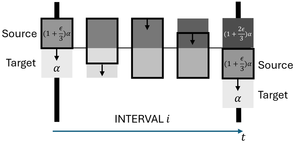
Our goal is to transform a given dynamic SC algorithm, denoted by $\mathcal{ALG}$ , that may have high worst-case recourse into one with low worst-case recourse, via a black-box transformation. To achieve this, we reduce our dynamic problem – of guaranteeing low worst-case recourse while preserving almost the same approximation and update time guarantees of the black-box $\mathcal{ALG}$ – to a static reconfiguration problem. The basic idea is to try and stick to the same output SC, changing it as little as possible to cope with element updates, until the approximation ratio deteriorates (a bit), at which stage we would need to switch the output SC to a better SC, but we must do it gradually rather than instantaneously. To this end, we shall run $\mathcal{ALG}$ in the “background”, and “sample” it for the output SC only periodically; we would like to gradually transform the current output SC (whose approximation has deteriorated) into the freshly sampled SC (whose approximation is good) throughout a sufficiently long time interval – as long as needed by the solution to the static reconfiguration problem.

Thus, we partition the update sequence into disjoint consecutive intervals, and at the start of each interval, the current output SC serves as the source solution, and the SC maintained by $\mathcal{ALG}$ serves as the target. We gradually transform the output from the source to the target during the interval; we would need to choose the interval lengths appropriately (see below), so that we will be able to complete the transformation process by the time the interval ends with a low worst-case recourse and with the required approximation guarantee. One hurdle in the dynamic setting that we completely ignored, which does not arise in the static reconfiguration problem, is that the element updates that occur during an interval may damage both the feasibility and approximation guarantee of the output SC. However, we show that the naive treatment of element updates for achieving feasibility has little effect on the approximation factor for small aspect ratio $C$ , and in general one can simply increase the recourse by a factor of $C$ .

2.3 Algorithm

Our algorithm will simulate $\mathcal{ALG}$ in the background. Denote by $T$ the worst-case update time of $\mathcal{ALG}$ . The update sequence will be divided into intervals. It begins with an “initial interval”, and then the first interval, the second interval, etc. We will denote the output solution, the background solution given by $\mathcal{ALG}$ , and an optimum solution, at the beginning of the $i$ -th interval by $\mathcal{X}_{i}$ , $\mathcal{B}_{i}$ and $\mathcal{OPT}_{i}$ , respectively. We define the initial interval as the $0$ -th interval, and we assume that $\mathcal{B}_{0}=\mathcal{X}_{0}$ . During the $i$ -th interval (for $i\geq 1$ ), we want to gradually transform the output from $\mathcal{X}_{i}$ to $\mathcal{B}_{i}$ . Since at the end of the $i$ -th interval $\mathcal{B}_{i}$ might no longer be a legal SC, for every element that is inserted during the interval, we add a set containing it to the output (this is not necessarily needed but in the worst-case this does occur so we assume so for simplicity). We define this as naively maintaining or naively extending the solution. We denote the collection of sets added naively during the $i$ -th interval as $\mathcal{N}_{i}$ . Thus, our goal is to gradually transform the output from $\mathcal{X}_{i}$ (source) to $(\mathcal{B}_{i}\cup\mathcal{N}_{i})$ (target) by the end of the $i$ -th interval.

To do so, we divide the $i$ -th interval (for $i\geq 1$ ) into two phases of equal length, the adding phase and the removing phase. In the adding phase we gradually add sets in $\mathcal{B}_{i}\setminus\mathcal{X}_{i}$ to the output, and in the removing phase we gradually remove sets in $\mathcal{X}_{i}\setminus\mathcal{B}_{i}$ from the output. In addition, as mentioned in the previous paragraph, during both phases we naively add one set per insertion. At the end of the second phase we have that $\mathcal{X}_{i+1}=(\mathcal{B}_{i}\cup\mathcal{N}_{i})$ .

The length of each phase in the $i$ -th interval will be $\left\lceil\frac{\epsilon}{12\alpha}\cdot\max\{\mathsf{cost}(\mathcal{X}_{i}),% \mathsf{cost}(\mathcal{B}_{i})\}\right\rceil$ update steps, so the length of the $i$ -th interval will be twice as long. We emphasize that the $i$ -th interval can also simply be of length $2\left\lceil\frac{\epsilon}{12\alpha}\cdot\mathsf{cost}(\mathcal{X}_{i})\right\rceil$ or $2\left\lceil\frac{\epsilon}{12\alpha}\cdot\mathsf{cost}(\mathcal{B}_{i})\right\rceil$ update steps (regardless of which is larger), and the theorem would still hold, but for the sake of consistency with Section 4 we take the maximum, which is necessary there. The initial interval will simply be of length $2\left\lceil\frac{\epsilon}{12\alpha}\cdot\mathsf{cost}(\mathcal{B}_{0})\right\rceil$ where at the end of it $\mathcal{X}_{1}=(\mathcal{B}_{0}\cup\mathcal{N}_{0})$ . To simplify the analysis, we assume that all terms within the ceilings are integers.

2.4 Analysis

Observation 5 (Recourse).

The worst-case recourse is $O(\frac{\alpha C}{\epsilon})$ .

Proof.

The worst-case recourse during the initial interval is one. In each phase in the $i$ -th interval ( $i\geq 1$ ) we gradually add or remove $\leq C\cdot\max\{\mathsf{cost}(\mathcal{X}_{i}),\mathsf{cost}(\mathcal{B}_{i})\}$ sets. This is done in up to $\frac{\epsilon}{12\alpha}\cdot\max\{\mathsf{cost}(\mathcal{X}_{i}),\mathsf{% cost}(\mathcal{B}_{i})\}$ update steps. We add one more set per insertion. $\hfill\blacktriangleleft$

Observation 6 (Update Time).

The worst-case update time is $T+O\left(\frac{\alpha C}{\epsilon}\right)$ .

Proof.

Three procedures contribute to the update time. The first is the update time of running $\mathcal{ALG}$ in the background, $T$ . The second is the gradual maintenance of the solution, with update time linear in that of the recourse. The third is choosing an arbitrary set containing an inserted element and adding it to the solution, which can be done in $O(1)$ time. $\hfill\blacktriangleleft$

Observation 7 (Legal Solution).

The output is always a valid SC (i.e., covers all elements).

Proof.

In the beginning of the $i$ -th interval we have two legal solutions, $\mathcal{X}_{i}$ and $\mathcal{B}_{i}$ . Throughout the $i$ -th interval the output solution always fully contains at least one of them, plus a set containing each inserted element. $\hfill\blacktriangleleft$ For the approximation factor, we will prove by induction on the intervals the following claim:

Claim 8 (Approximation Factor).

For any $i\geq 0$ :

1.

The approximation factor of the output solution throughout the $i$ -th interval is $(2+\epsilon)\cdot\alpha$ .
2.

The approximation factor of the output solution at the beginning of the $(i+1)$ -th interval is $(1+\frac{\epsilon}{3})\cdot\alpha$ .

2.4.1 Proof of Claim 8

In this section we prove Claim 8. Theorem 1 would hold by Observation 5, Observation 6, Observation 7 and Claim 8 (1). For any $i\geq 0$ , denote the output solution, the background solution given by $\mathcal{ALG}$ , and an optimum solution, $t$ update steps after the beginning of the $i$ -th interval until it ends, by $\mathcal{X}_{i}^{t}$ , $\mathcal{B}_{i}^{t}$ and $\mathcal{OPT}_{i}^{t}$ , respectively. For the highest possible $t$ (given a specific $i$ ) we have $\mathcal{X}_{i}^{t}=\mathcal{X}_{i+1}$ , $\mathcal{B}_{i}^{t}=\mathcal{B}_{i+1}$ and $\mathcal{OPT}_{i}^{t}=\mathcal{OPT}_{i+1}$ . We begin with the following observation:

Observation 9.

In each update step the cost of the output can increase by at most $1$ , since the cost of sets lies in the range $[\frac{1}{C},1]$ . Similarly, in each update step the cost of the optimum can decrease by up to $1$ , since only one set can leave an optimum solution each update step (and its cost is upper bounded by $1$ ).

We begin by proving the base case.

Observation 10.

For any $t$ we have that $\mathsf{cost}(\mathcal{X}_{0}^{t})\leq\mathsf{cost}(\mathcal{X}_{0})+\frac{% \epsilon}{6}\cdot\mathsf{cost}(\mathcal{OPT}_{0})$ and $\mathsf{cost}(\mathcal{OPT}_{0}^{t})\geq(1-\frac{\epsilon}{6})\cdot\mathsf{% cost}(\mathcal{OPT}_{0})$ .

Proof.

By Observation 9:

\mathsf{cost}(\mathcal{X}_{0}^{t})\leq\mathsf{cost}(\mathcal{X}_{0})+\frac{% \epsilon}{6\alpha}\cdot\mathsf{cost}(\mathcal{B}_{0})\leq\mathsf{cost}(% \mathcal{X}_{0})+\frac{\epsilon}{6}\cdot\mathsf{cost}(\mathcal{OPT}_{0}).

Similarly, by Observation 9:

\mathsf{cost}(\mathcal{OPT}_{0}^{t})\geq\mathsf{cost}(\mathcal{OPT}_{0})-\frac% {\epsilon}{6\alpha}\cdot\mathsf{cost}(\mathcal{B}_{0})\geq\mathsf{cost}(% \mathcal{OPT}_{0})-\frac{\epsilon}{6}\cdot\mathsf{cost}(\mathcal{OPT}_{0}).\

$\hfill\blacktriangleleft$

Observation 11.

The approximation factor $t$ update steps after the beginning of the initial interval and until it ends is $(1+\frac{\epsilon}{3})\cdot\alpha$ .

Proof.

By Observation 10 we get that:

\begin{array}[]{rcl}\displaystyle\frac{\mathsf{cost}(\mathcal{X}_{0}^{t})}{% \mathsf{cost}(\mathcal{OPT}_{0}^{t})}&\leq&\displaystyle\frac{\mathsf{cost}(% \mathcal{X}_{0})+\frac{\epsilon}{6}\cdot\mathsf{cost}(\mathcal{OPT}_{0})}{(1-% \frac{\epsilon}{6})\cdot\mathsf{cost}(\mathcal{OPT}_{0})}\\[11.38109pt] &\leq&\displaystyle\frac{(\alpha+\frac{\epsilon}{6})\cdot\mathsf{cost}(% \mathcal{OPT}_{0})}{(1-\frac{\epsilon}{6})\cdot\mathsf{cost}(\mathcal{OPT}_{0}% )}\\[11.38109pt] &=&\displaystyle\frac{\alpha+\frac{\epsilon}{6}}{1-\frac{\epsilon}{6}}\\[11.38% 109pt] &\leq&(1+\frac{\epsilon}{3})\cdot\alpha,\end{array}

where the last inequality holds for any $\epsilon<1$ and $\alpha\geq 2$ . $\hfill\blacktriangleleft$ We have shown that both items of Claim 8 hold for the base case ( $i=0$ ). For the induction step, we begin with the first item:

Observation 12.

The approximation factor $t$ update steps after the beginning of the $i$ -th interval and until it ends is $(2+\epsilon)\cdot\alpha$ .

Proof.

\begin{array}[]{rcl}\displaystyle\frac{\mathsf{cost}(\mathcal{X}_{i}^{t})}{% \mathsf{cost}(\mathcal{OPT}_{i}^{t})}&\leq&\displaystyle\frac{\mathsf{cost}(% \mathcal{X}_{i})+\mathsf{cost}(\mathcal{B}_{i})+\frac{\epsilon}{6\alpha}\cdot% \max\{\mathsf{cost}(\mathcal{X}_{i}),\mathsf{cost}(\mathcal{B}_{i})\}}{\mathsf% {cost}(\mathcal{OPT}_{i})-\frac{\epsilon}{6\alpha}\cdot\max\{\mathsf{cost}(% \mathcal{X}_{i}),\mathsf{cost}(\mathcal{B}_{i})\}}\\[11.38109pt] &\leq&\displaystyle\frac{(1+\frac{\epsilon}{3})\cdot\alpha+\alpha+\frac{% \epsilon}{6}\cdot(1+\frac{\epsilon}{3})}{1-\frac{\epsilon}{6}\cdot(1+\frac{% \epsilon}{3})}\\[11.38109pt] &\leq&(2+\epsilon)\cdot\alpha,\end{array}

where the first inequality is by Observation 9, the second by the induction hypothesis (Claim 8 (2)), and the last holds for any $\epsilon\leq 0.7$ and $\alpha\geq 2$ . $\hfill\blacktriangleleft$

Observation 13.

At the beginning of the $(i+1)$ -th interval, the approximation factor is $(1+\frac{\epsilon}{3})\cdot\alpha$ .

Proof.

\begin{array}[]{rcl}\displaystyle\frac{\mathsf{cost}(\mathcal{X}_{i+1})}{% \mathsf{cost}(\mathcal{OPT}_{i+1})}&\leq&\displaystyle\frac{\mathsf{cost}(% \mathcal{B}_{i})+\frac{\epsilon}{6\alpha}\cdot\max\{\mathsf{cost}(\mathcal{X}_% {i}),\mathsf{cost}(\mathcal{B}_{i})\}}{\mathsf{cost}(\mathcal{OPT}_{i})-\frac{% \epsilon}{6\alpha}\cdot\max\{\mathsf{cost}(\mathcal{X}_{i}),\mathsf{cost}(% \mathcal{B}_{i})\}}\\[11.38109pt] &\leq&\displaystyle\frac{\alpha+\frac{\epsilon}{6}\cdot(1+\frac{\epsilon}{3})}% {1-\frac{\epsilon}{6}\cdot(1+\frac{\epsilon}{3})}\\[11.38109pt] &\leq&(1+\frac{\epsilon}{3})\cdot\alpha,\end{array}

where the first inequality is by Observation 9, the second by the induction hypothesis (Claim 8 (2)), and the last holds for any $\epsilon\leq 0.5$ and $\alpha\geq 2$ . $\hfill\blacktriangleleft$ See Figure 1 for an illustration of the black-box transformation. We have shown that both items of Claim 8 hold for the induction step, concluding its proof. This completes the proof of Theorem 1.

Refer to caption — Figure 1: The $i$ -th interval, showing the source solution (top square) and target solution (bottom square), where darker shades represent a higher (worse) approximation ratio. The output (black rectangle contour) is constructed from the union of both. At the start of the interval, the output solution is identical to the source, which provides a $(1+\frac{\epsilon}{3})\alpha$ -approximation, while the target provides an $\alpha$ -approximation by $\mathcal{ALG}$ . During the interval, the target is gradually added to the output; once it is contained, the source is gradually removed. Although the approximation factor of each solution degrades over time – starting at light gray ( $\alpha$ ) and eventually becoming dark gray ( $(1+\frac{2\epsilon}{3})\alpha$ ) – the union of the source and target maintains a $(2+\epsilon)\alpha$ -approximation throughout. The output at the end of the interval becomes the source for the next interval, and the solution given by $\mathcal{ALG}$ at that point becomes the next target.

3 The Robustness Property

The main result of this section is Lemma 16, which asserts that the greedy-based dynamic algorithm of [41] is robust. This robustness property is crucial for shaving off the $\log n$ term from the recourse, thereby proving Theorem 3 (see Section 4 for details). We begin in Section 3.1 by observing (Observation 14) that the classic static greedy algorithm produces a robust SC whereas the classic static PD algorithm is not robust. While Observation 14 serves as a warm-up for the dynamic robustness lemma (Lemma 16), it may also be of independent interest.

3.1 The Robustness Property I: The Greedy and PD Static Algorithms

Observation 14 (Warm-up: Static greedy is robust).

Let $(\mathcal{U},\mathcal{S})$ be any set system and let $X$ be a SC returned by the classic greedy algorithm, and $\mathsf{OPT}$ the optimum value. Let $\mathcal{D}\subseteq\mathcal{U}$ be any set of deleted elements with $|\mathcal{D}|\leq\delta\cdot\mathsf{cost}(X)$ for any $0<\delta<1$ , and let $\mathsf{OPT^{\prime}}$ be the optimum value after these deletions. Then:

\frac{\mathsf{cost}(X)}{\mathsf{OPT^{\prime}}}\;\leq\;\frac{H_{n}}{1-\delta}\;% \leq\;(1+O(\delta))\,\ln n,

where $n:=|\mathcal{U}|$ and $H_{n}$ is the $n$ -th harmonic number.

Proof.

As the greedy algorithm selects a set $s$ that newly covers a set of elements $u(s)$ , assign to each such element $e\in u(s)$ a weight:

q(e):=\frac{\mathsf{cost}(s)}{|u(s)|}.

The total cost of the greedy solution equals the sum of assigned weights:

\sum_{e\in\mathcal{U}}q(e)=\mathsf{cost}(X).

Since $\mathsf{cost}(s)\leq 1$ and $|u(s)|\geq 1$ , we have $q(e)\leq 1$ for all $e$ . Define the restricted weights $q^{\prime}(e)$ to be $0$ if $e\in\mathcal{D}$ and $q(e)$ otherwise. Then:

\hfill\mathsf{cost}(X)=\sum_{e\in\mathcal{U}\setminus\mathcal{D}}q(e)+\sum_{e% \in\mathcal{D}}q(e)\leq\sum_{e\in\mathcal{U}}q^{\prime}(e)+|\mathcal{D}|\leq% \sum_{e\in\mathcal{U}}q^{\prime}(e)+\delta\cdot\mathsf{cost}(X).\hfill

(1)

Now, let $\{s_{1},s_{2},\ldots,s_{k}\}$ be the sets in an optimal set cover for the system after deletions $(\mathcal{U}\setminus\mathcal{D},\mathcal{S})$ . Consider one such set $s_{i}$ . Let the elements of $s_{i}$ be $\{e_{1},e_{2},\ldots,e_{x_{i}}\}$ , ordered by when they were covered by the greedy algorithm.

Claim 15.

For any $e_{j}\in s_{i}\setminus\mathcal{D}$ , we have $q^{\prime}(e_{j})\leq\frac{\mathsf{cost}(s_{i})}{x_{i}-j+1}$ .

Proof.

At the step where the greedy algorithm covers $e_{j}$ using some set $s$ , the elements $\{e_{j},e_{j+1},\ldots,e_{x_{i}}\}$ are all still uncovered. Thus, at that point, the set $s_{i}$ contains at least $x_{i}-j+1$ uncovered elements. Since the greedy algorithm picks a set $s$ to minimize the cost-per-newly-covered-element ratio:

q(e_{j})=\frac{\mathsf{cost}(s)}{|u(s)|}\leq\frac{\mathsf{cost}(s_{i})}{x_{i}-% j+1}.

As $q^{\prime}(e_{j})=q(e_{j})$ for $e_{j}\notin\mathcal{D}$ , the claim follows. $\hfill\vartriangleleft$ Summing the weights for all elements in $s_{i}$ that were not deleted:

\sum_{e\in s_{i}\setminus\mathcal{D}}q^{\prime}(e)\leq\sum_{j=1}^{x_{i}}\frac{% \mathsf{cost}(s_{i})}{x_{i}-j+1}=\mathsf{cost}(s_{i})\cdot H_{x_{i}}\leq% \mathsf{cost}(s_{i})\cdot H_{n}.

By summing over all $k$ sets in the optimal solution $\mathsf{OPT^{\prime}}$ :

\hfill\sum_{i=1}^{k}\sum_{e\in s_{i}\setminus\mathcal{D}}q^{\prime}(e)\leq\sum% _{i=1}^{k}\mathsf{cost}(s_{i})\cdot H_{n}=\mathsf{OPT^{\prime}}\cdot H_{n}.\hfill

(2)

Since the optimal solution covers all elements in $\mathcal{U}\setminus\mathcal{D}$ , we have:

\hfill\sum_{e\in\mathcal{U}}q^{\prime}(e)\leq\sum_{i=1}^{k}\sum_{e\in s_{i}% \setminus\mathcal{D}}q^{\prime}(e).\hfill

(3)

Combining (1), (2), and (3) concludes the proof. $\hfill\blacktriangleleft$

Remark.

Replacing $H_{n}$ with $H_{d}$ , where $d=\max_{s\in\mathcal{S}}|s|$ , gives:

\frac{\mathsf{cost}(X)}{\mathsf{OPT^{\prime}}}\leq\frac{H_{d}}{1-\delta}\leq(1% +O(\delta))\ln d.

The classic PD algorithm is not robust.

Consider the following canonical unweighted instance: For each element $e_{i}$ , where $i=1,\ldots,n$ , create $f$ sets $S^{1}_{i},\ldots,S^{f}_{i}$ that contain only $e_{i}$ . The PD algorithm could add all $n\cdot f$ sets to the SC, while $\mathsf{OPT}$ has size $n$ . If $\ell$ elements are deleted, for any $\ell$ , we have $|\mathsf{OPT}|=n-\ell$ . In particular, for $\ell=n-O(1)$ (the extreme case being $\ell=n$ ), $\mathsf{OPT}$ is of size $O(1)$ (or 0); thus already for $\delta=1/f$ , after deleting a $\delta$ fraction of the elements in the solution produced by the PD algorithm, the approximation may become arbitrarily large, thus the PD algorithm is not robust (and actually far from robust). Furthermore, if $\ell=n-O(1)$ , we will need to delete $n\cdot f-A$ sets from the set cover to achieve an approximation factor of $O(A)$ , which gives an amortized recourse of $\Omega(f)$ for any reasonable approximation. This shows the asymptotic optimality of the recourse bound provided by Corollary 2 (for constant $C$ and $\delta$ ): any PD-based algorithm must have a recourse of $\Omega(f)$ , even in the amortized sense and the decremental-only setting.

Although this example with singleton sets is degenerate, since there is no incentive to include multiple sets to cover the same element, this can be extended to less degenerate instances with more dummy sets and elements. The key point remains: the fact that a sequence of deletions can cause $|\mathsf{OPT}|$ to drop significantly does not imply that the initial approximation was strictly better than $f$ , in contrast to the greedy algorithm, as seen in Observation 14.

3.2 The Robustness Property II: The Dynamic Algorithm [41]

In this section we prove that the greedy-based algorithm of [41] is robust. In fact, we prove a stronger variant: the algorithm is also “robust against insertions”, as defined below.

Lemma 16 ([41] is Robust - Greedy-Based).

Consider a solution given by [41] denoted by $\mathcal{B}$ , yielding an approximation factor of $(1+\epsilon)\cdot\ln n$ . Then throughout the next $\delta\cdot\mathsf{cost}(\mathcal{B})$ update steps (for any $0\leq\delta\leq 1$ ) during which we maintain $\mathcal{B}$ naively (adding an arbitrary set containing each inserted element to it), the approximation factor is $(1+O(\delta))(1+\epsilon)\cdot\ln n$ .

3.2.1 Preliminaries

We first review the primary definitions from [41]. Let $\beta=1+\epsilon$ . All sets $s\in\mathcal{S}$ are assigned a level value $\mathsf{lev}(s)\in[-1,L]$ where $L=\lceil\log_{\beta}(Cn)\rceil+\lceil 10\log_{\beta}1/\epsilon\rceil$ . Throughout the algorithm, a valid set cover $\mathcal{B}\subseteq\mathcal{S}$ is maintained for all elements. Each element $e\in\mathcal{U}$ is assigned to one of the sets $s\in\mathcal{B}$ , which we denote by $\mathsf{asn}(e)$ , and conversely, for each set $s\in\mathcal{S}$ , define its covering set $\mathsf{cov}(s)$ to be the collection of elements in $s$ that are assigned to $s$ , namely $\mathsf{cov}(s)=\{e\mid\mathsf{asn}(e)=s\}$ . The level of an element $e$ is defined as the level of the set it is assigned to, namely $\mathsf{lev}(e)=\mathsf{lev}(\mathsf{asn}(e))$ , and we are guaranteed that $\mathsf{lev}(e)=\max\{lev(s)|s\ni e\}$ , i.e., $e$ is assigned to the highest-level set containing it. We define the level of each set $s\notin\mathcal{B}$ to be $-1$ , whereas the level of each set $s\in\mathcal{B}$ will lie in $[0,L]$ , so in particular we will have $\mathsf{lev}(e)\in[0,L]$ , for each element $e\in\mathcal{U}$ . Let $S_{i}=\{s\mid\mathsf{lev}(s)=i\},\forall i\in[-1,L]$ , and $E_{i}=\{e\in\mathcal{U}\mid\mathsf{lev}(e)=i\},\forall i\in[0,L]$ .

Besides the level value $\mathsf{lev}(e)$ for elements $e$ , a value of passive level $\mathsf{plev}(e)$ such that $\mathsf{lev}(e)\leq\mathsf{plev}(e)\leq L$ is also maintained, which is central to the algorithm. In contrast to the level $\mathsf{lev}(e)$ of an element $e$ , which may decrease (as well as increase) by the algorithm, its passive level $\mathsf{plev}(e)$ is monotonically non-decreasing throughout its lifespan.

An element is said to be dead if it was deleted by the adversary, hence it should be removed from $\mathcal{U}$ , yet it remains in $\mathcal{U}^{+}$ because the algorithm has not yet “processed” the deletion. An element is said to be alive if it is not dead. To avoid confusion, the notation $\mathcal{U}^{+}\supseteq\mathcal{U}$ is used to denote the set of all dead and alive elements (i.e., the elements from the algorithm’s perspective), while $\mathcal{U}$ is the set of alive elements (i.e., the elements from the adversary’s perspective). We next introduce the following key definitions.

Definition 17.

For each level $k$ , an element $e\in\mathcal{U}^{+}$ is called $k$ -active (respectively, $k$ -passive) if $\mathsf{lev}(e)\leq k<\mathsf{plev}(e)$ (resp., $\mathsf{plev}(e)\leq k$ ) and let $A_{k}=\{e\in\mathcal{U}^{+}\mid\mathsf{lev}(e)\leq k<\mathsf{plev}(e)\}$ and $P_{k}=\{e\in\mathcal{U}^{+}\mid\mathsf{plev}(e)\leq k\}$ be the sets of all $k$ -active and $k$ -passive elements, respectively. Notice that $A_{k}\cup P_{k}$ is the collection of all elements at level $\leq k$ , and $A_{k}\cap P_{k}=\emptyset$ . Moreover, if $A_{k}\cap P_{j}\neq\emptyset$ for two levels $k\neq j$ , then $k<j$ . For each set $s\in\mathcal{S}$ , define $N_{k}(s)=A_{k}\cap s$ .

3.2.2 Invariants

The algorithm of [41] maintains the following three invariants. The first and second are identical to those presented in [41], but the third here is a relaxed version of the third there, which originally demanded that for each $k\in[0,L]$ , we have $|P_{k}|\leq 2\epsilon\cdot|A_{k}|$ . This relaxation is crucial for the robustness proof.

1.

For any set $s\in\mathcal{S}$ and for each $k\in[0,L]$ , we have $\frac{|N_{k}(s)|}{\mathsf{cost}(s)}<\beta^{k+1}$ .
2.

For any set $s\in\mathcal{B}$ , we have $\frac{|\mathsf{cov}(s)|}{\mathsf{cost}(s)}\geq\beta^{\mathsf{lev}(s)}$ ; we note that $\mathsf{cov}(s)$ may include dead elements, i.e., elements in $\mathcal{U}^{+}\setminus\mathcal{U}$ . In particular, $\mathsf{lev}(s)\leq\lceil\log_{\beta}(Cn)\rceil$ . Moreover, for each $s\notin\mathcal{B}$ , $\mathsf{lev}(s)=-1$ .
3.

$\sum_{k=0}^{L-1}\left(\beta^{-k}-\beta^{-k-1}\right)\cdot|P_{k}|\leq 2\epsilon% \cdot\sum_{k=0}^{L-1}\left(\beta^{-k}-\beta^{-k-1}\right)\cdot|A_{k}|.$

3.2.3 Proof of Lemma 16

For the most part, the proof of Lemma 16 follows the proof of the approximation factor in [41], except in one key area. We will present the entire formal proof and state exactly where this deviation occurs. Specifically, the first and third parts will be similar to [41], whereas the second part will be new.

Part I – Similar to [41].

The left-hand side of the third invariant can be rewritten as:

	$\displaystyle\sum_{k=0}^{L-1}(\beta^{-k}-\beta^{-k-1})\cdot\|P_{k}\|$	$\displaystyle=\sum_{e\in\mathcal{U}^{+}}\sum_{k=0}^{L-1}(\beta^{-k}-\beta^{-k-% 1})\cdot\mathbf{1}[e\in P_{k}]$
		$\displaystyle=\sum_{e\in\mathcal{U}^{+}}\sum_{k=\mathsf{plev}(e)}^{L-1}(\beta^% {-k}-\beta^{-k-1})$
		$\displaystyle=\sum_{e\in\mathcal{U}^{+}}\left(\beta^{-\mathsf{plev}(e)}-\beta^% {-L}\right)$

and the right-hand side of the third invariant can be rewritten as:

	$\displaystyle 2\epsilon\sum_{k=0}^{L-1}(\beta^{-k}-\beta^{-k-1})\cdot\|A_{k}\|$	$\displaystyle=2\epsilon\sum_{e\in\mathcal{U}^{+}}\sum_{k=0}^{L-1}(\beta^{-k}-% \beta^{-k-1})\cdot\mathbf{1}[e\in A_{k}]$
		$\displaystyle=2\epsilon\sum_{e\in\mathcal{U}^{+}}\sum_{k=\mathsf{lev}(e)}^{% \mathsf{plev}(e)-1}(\beta^{-k}-\beta^{-k-1})$
		$\displaystyle=2\epsilon\sum_{e\in\mathcal{U}^{+}}\left(\beta^{-\mathsf{lev}(e)% }-\beta^{-\mathsf{plev}(e)}\right),$

which yields:

\sum_{e\in\mathcal{U}^{+}}\left(\beta^{-\mathsf{plev}(e)}-\beta^{-L}\right)% \leq 2\epsilon\cdot\sum_{e\in\mathcal{U}^{+}}\left(\beta^{-\mathsf{lev}(e)}-% \beta^{-\mathsf{plev}(e)}\right)

or equivalently, by adding $\sum_{e\in\mathcal{U}^{+}}\left(\beta^{-\mathsf{lev}(e)}-\beta^{-\mathsf{plev}% (e)}\right)$ to both sides:

\hfill\sum_{e\in\mathcal{U}^{+}}\left(\beta^{-\mathsf{lev}(e)}-\beta^{-L}% \right)\nobreak\ \leq\nobreak\ (1+2\epsilon)\cdot\sum_{e\in\mathcal{U}^{+}}% \left(\beta^{-\mathsf{lev}(e)}-\beta^{-\mathsf{plev}(e)}\right).\hfill

(4)

We emphasize the point that $\mathcal{U}^{+}$ also includes dead elements. We also have that:

	$\displaystyle\mathsf{cost}(\mathcal{B})$	$\displaystyle=\sum_{s\in\mathcal{B}}\mathsf{cost}(s)\leq\sum_{s\in\mathcal{B}}% \beta^{-\mathsf{lev}(s)}\cdot\|\mathsf{cov}(s)\|\nobreak\ =\nobreak\ \beta\cdot% \sum_{s\in\mathcal{B}}\sum_{e\in\mathsf{cov}(s)\cap\mathcal{U}^{+}}\beta^{-% \mathsf{lev}(e)}$		(5)
		$\displaystyle\leq(1+O(\epsilon))\cdot\sum_{e\in\mathcal{U}^{+}}\left(\beta^{-% \mathsf{lev}(e)}-\beta^{-L}\right),$		(5)

where the first inequality holds by the second invariant and the second holds as $\mathsf{lev}(e)\leq L/2$ and hence $\beta^{-\mathsf{lev}(e)}-\beta^{-L}\geq\beta^{-\mathsf{lev}(e)}(1-\beta^{-% \lceil 10\log_{\beta}1/\epsilon\rceil})\geq\beta^{-\mathsf{lev}(e)}(1-\varepsilon)$ . Combining Equation 4 and Equation 5 we obtain:

\hfill\mathsf{cost}(\mathcal{B})\nobreak\ \leq\nobreak\ (1+O(\epsilon))\cdot% \sum_{e\in\mathcal{U}^{+}}\left(\beta^{-\mathsf{lev}(e)}-\beta^{-\mathsf{plev}% (e)}\right).\hfill

(6)

Part II – New Ideas.

Our goal will be to show that following $\delta\cdot\mathsf{cost}(\mathcal{B})$ updates we have:

\hfill\mathsf{cost}(\mathcal{B})\nobreak\ \leq\nobreak\ (1+O(\delta))(1+O(% \epsilon))\cdot\sum_{e\in\mathcal{U}^{+}}\left(\beta^{-\mathsf{lev}(e)}-\beta^% {-\mathsf{plev}(e)}\right).\hfill

(7)

The most adverse effect of an insertion is an increase in the cost of the maintained set cover by one. Conversely, the most significant reduction to the right-hand side of Equation 6 occurs if a deleted element’s passive level drops from the maximum level to zero. We will first handle the deletions. By $\delta\cdot\mathsf{cost}(\mathcal{B})$ deletions, the right-hand side of Equation 6 can be lowered only by less than $(1+O(\epsilon))\cdot\delta\cdot\mathsf{cost}(\mathcal{B})$ . This is because for each deleted element $e$ , $\beta^{-\mathsf{plev}(e)}$ can rise only by less than $1$ , and the rest does not change. Thus, after the $\delta\cdot\mathsf{cost}(\mathcal{B})$ deletions, we can claim that:

\hfill\mathsf{cost}(\mathcal{B})\nobreak\ \leq\nobreak\ (1+O(\epsilon))\cdot% \sum_{e\in\mathcal{U}^{+}}\left(\beta^{-\mathsf{lev}(e)}-\beta^{-\mathsf{plev}% (e)}\right)+(1+O(\epsilon))\cdot\delta\cdot\mathsf{cost}(\mathcal{B}).\hfill

(8)

Rearranging, and for any $\delta\leq 1$ , we indeed get that Equation 7 holds. Regarding the insertions, in the worst-case $\mathsf{cost}(\mathcal{B})$ grew by a factor of $(1+\delta)$ , since the cost of each set is no more than $1$ . Clearly Equation 7 would still hold (by multiplying the right-hand side of Equation 7 by $(1+\delta)$ ).

Part III – Similar to [41].

Denote by $\mathcal{S}^{*}$ an optimum SC. Next, let us lower bound $\mathsf{cost}(\mathcal{S}^{*})$ using the term $\sum_{e\in\mathcal{U}^{+}}\left(\beta^{-\mathsf{lev}(e)}-\beta^{-\mathsf{plev}% (e)}\right)$ . For any $s\in\mathcal{S}^{*}$ , consider the following three cases for any index $k\in[L]$ :

$\blacksquare$

$k<\log_{\beta}(1/\mathsf{cost}(s))-1$ .

By the first invariant, we have: $|N_{k}(s)|<\beta^{k+1}\cdot\mathsf{cost}(s)<1$ , so $|N_{k}(s)|=0$ .
$\blacksquare$

$\log_{\beta}(1/\mathsf{cost}(s))-1\leq k\leq\log_{\beta}(n/\mathsf{cost}(s))$ .

By the first invariant, we have:

$\frac{1}{\epsilon}\left(\beta^{-k}-\beta^{-k-1}\right)|N_{k}(s)|=\beta^{-k-1}|% N_{k}(s)|<\mathsf{cost}(s).$
$\blacksquare$

$k>\lceil\log_{\beta}(n/\mathsf{cost}(s))\rceil=k_{0}$ .

In this case, we use the trivial bound: $|N_{k}(s)|\leq n\leq\beta^{k_{0}}\cdot\mathsf{cost}(s)$ , and so we have:

$\frac{1}{\epsilon}\left(\beta^{-k}-\beta^{-k-1}\right)|N_{k}(s)|=\beta^{-k-1}|% N_{k}(s)|\leq\beta^{k_{0}-k-1}\cdot\mathsf{cost}(s).$

Observe that:

$\displaystyle\frac{1}{\epsilon}\sum_{k=0}^{L-1}(\beta^{-k}-\beta^{-k-1})\cdot\|% N_{k}(s)\|$	$\displaystyle=\frac{1}{\epsilon}\sum_{e\in s}\sum_{k=0}^{L-1}(\beta^{-k}-\beta% ^{-k-1})\cdot\mathbf{1}[e\in N_{k}(s)]$	(9)
	$\displaystyle=\frac{1}{\epsilon}\sum_{e\in s}\sum_{k=\mathsf{lev}(e)}^{\mathsf% {plev}(e)-1}(\beta^{-k}-\beta^{-k-1})$
	$\displaystyle=\frac{1}{\epsilon}\sum_{e\in s}\left(\beta^{-\mathsf{lev}(e)}-% \beta^{-\mathsf{plev}(e)}\right).$

By the above case analysis, we have:

$\displaystyle\frac{1}{\epsilon}\sum_{k=0}^{L-1}(\beta^{-k}-\beta^{-k-1})\cdot\|% N_{k}(s)\|$	$\displaystyle=\frac{1}{\epsilon}\sum_{0\leq k<\log_{\beta}(1/\mathsf{cost}(s))% -1}(\beta^{-k}-\beta^{-k-1})\cdot\|N_{k}(s)\|$	(10)
	$\displaystyle\nobreak\ \nobreak\ \nobreak\ +\frac{1}{\epsilon}\sum_{\log_{% \beta}(1/\mathsf{cost}(s))-1\leq k\leq\log_{\beta}(n/\mathsf{cost}(s))}(\beta^% {-k}-\beta^{-k-1})\cdot\|N_{k}(s)\|$
	$\displaystyle\nobreak\ \nobreak\ \nobreak\ +\frac{1}{\epsilon}\sum_{\log_{% \beta}(n/\mathsf{cost}(s))<k\leq L-1}(\beta^{-k}-\beta^{-k-1})\cdot\|N_{k}(s)\|$
	$\displaystyle<\sum_{0\leq k<\log_{\beta}(1/\mathsf{cost}(s))-1}0$
	$\displaystyle\nobreak\ \nobreak\ \nobreak\ +\sum_{\log_{\beta}(1/\mathsf{cost}% (s))-1\leq k\leq\log_{\beta}(n/\mathsf{cost}(s))}\mathsf{cost}(s)$
	$\displaystyle\nobreak\ \nobreak\ \nobreak\ +\sum_{\log_{\beta}(n/\mathsf{cost}% (s))<k\leq L-1}\beta^{k_{0}-k-1}\mathsf{cost}(s)$
	$\displaystyle<\left(0+(\log_{\beta}(n)+2)+1/\epsilon\right)\cdot\mathsf{cost}(% s).$

Combining Equation 9 with Equation 10 yields

\frac{1}{\epsilon}\sum_{e\in s}\left(\beta^{-\mathsf{lev}(e)}-\beta^{-\mathsf{% plev}(e)}\right)\leq\left(\log_{\beta}(n)+2+1/\epsilon\right)\cdot\mathsf{cost% }(s).

Therefore, as $\ln(1+\epsilon)=\epsilon+O(\epsilon^{2})$ , under the assumption that $\varepsilon=\Omega(1/\log n)$ we have:

\sum_{e\in s}\left(\beta^{-\mathsf{lev}(e)}-\beta^{-\mathsf{plev}(e)}\right)% \leq(1+O(\epsilon))\ln n\cdot\mathsf{cost}(s).

Since $\mathcal{S}^{*}$ is a valid set cover for all elements in $\mathcal{U}$ (all the alive elements) and as for each dead element $e$ (in $\mathcal{U}^{+}\setminus\mathcal{U}$ ) we have $\left(\beta^{-\mathsf{lev}(e)}-\beta^{-\mathsf{plev}(e)}\right)=0$ , it follows that:

\sum_{e\in\mathcal{U}^{+}}\left(\beta^{-\mathsf{lev}(e)}-\beta^{-\mathsf{plev}% (e)}\right)\nobreak\ \leq\nobreak\ \sum_{s\in S^{*}}\sum_{e\in s}(\beta^{-% \mathsf{lev}(e)}-\beta^{-\mathsf{plev}(e)})\nobreak\ \leq\nobreak\ (1+O(% \epsilon))\ln n\cdot\mathsf{cost}(\mathcal{S}^{*}).

(11)

We conclude that:

	$\displaystyle\mathsf{cost}(\mathcal{B})$	$\displaystyle\leq(1+O(\delta))(1+O(\epsilon))\cdot\sum_{e\in\mathcal{U}^{+}}% \left(\beta^{-\mathsf{lev}(e)}-\beta^{-\mathsf{plev}(e)}\right)$
		$\displaystyle\leq(1+O(\delta))(1+O(\epsilon))\ln n\cdot\mathsf{cost}(\mathcal{% S}^{*}),$

where the first inequality holds by Equation 7 and the second by Equation 11. By scaling $\epsilon$ , we conclude the proof of Lemma 16.

4 Worst-Case Recourse: $O\left(\frac{\log n\cdot C}{\epsilon}\right)$ to $O\left(\frac{C}{\epsilon}\right)$ (Greedy)

This section is devoted to the proof of Theorem 3. We begin by recalling the main greedy-based result obtained by [41]:

Theorem 18 ([41] – Greedy-Based).

For any set system $(\mathcal{U},\mathcal{S})$ that undergoes a sequence of element insertions and deletions, where the frequency is bounded by $f$ , and for any $\epsilon\in(0,\frac{1}{4})$ , there is a deterministic algorithm that maintains a $((1+\epsilon)\ln n)$ -approximate SC in $O\left(\frac{f\log n}{\epsilon^{2}}\right)$ worst-case update time.

Applying this algorithm to our black-box transformation presented in Section 2 yields a $((2+\epsilon)\ln n)$ -approximate SC in $O\left(\frac{f\cdot\log n}{\epsilon^{2}}+\frac{\log n\cdot C}{\epsilon}\right)$ worst-case update time and with a worst-case recourse of $O\left(\frac{\log n\cdot C}{\epsilon}\right)$ . Our goal is to remove the $\log n$ factor from the recourse bound. The core strategy is to scale the interval lengths as defined in Section 2 by a factor of $\ln n$ to reduce the recourse, while leveraging the robustness property established in Section 3.2 to ensure the approximation ratio remains bounded. However, the situation is much more subtle, since the robustness of a SC solution depends on its cost, while the costs of the source and target solutions at the start and end of each interval may differ by a factor of $\ln n$ . This subtlety necessitates a considerably more refined analysis, detailed in Section 4.2.

4.1 Algorithm Description

We employ the exact same algorithm as in Section 2, with the sole modification being that interval lengths are increased by a factor of $\alpha=\ln n$ . Specifically, the length of the $i$ -th interval will be $2\left\lceil\frac{\epsilon}{12}\cdot\max\{\mathsf{cost}(\mathcal{X}_{i}),% \mathsf{cost}(\mathcal{B}_{i})\}\right\rceil$ update steps, and each phase will consist of $\left\lceil\frac{\epsilon}{12}\cdot\max\{\mathsf{cost}(\mathcal{X}_{i}),% \mathsf{cost}(\mathcal{B}_{i})\}\right\rceil$ update steps. The initial interval will have a length of $2\left\lceil\frac{\epsilon}{12}\cdot\mathsf{cost}(\mathcal{B}_{0})\right\rceil$ update steps. To simplify the analysis, we assume that all terms within the ceilings are integers.

Observation 19 (Recourse).

The worst-case recourse is $O(\frac{C}{\epsilon})$ .

Proof.

The worst-case recourse during the initial interval is one. In each phase in the $i$ -th interval ( $i\geq 1$ ) we gradually add or remove $\leq C\cdot\max\{\mathsf{cost}(\mathcal{X}_{i}),\mathsf{cost}(\mathcal{B}_{i})\}$ sets. This is done in up to $\frac{\epsilon}{12}\cdot\max\{\mathsf{cost}(\mathcal{X}_{i}),\mathsf{cost}(% \mathcal{B}_{i})\}$ update steps. We add one more set per insertion. $\hfill\blacktriangleleft$

Observation 20 (Update Time).

The worst-case update time is $O\left(\frac{f\cdot\log n}{\epsilon^{2}}+\frac{C}{\epsilon}\right)$ .

Proof.

Three procedures contribute to the update time. The first is the update time of running [41] in the background, $O\left(\frac{f\log n}{\epsilon^{2}}\right)$ . The second is the gradual maintenance of the solution, with update time linear in that of the recourse. The third is choosing an arbitrary set containing an inserted element and adding it to the solution, which can be done in $O(1)$ time. $\hfill\blacktriangleleft$

Observation 21 (Legal Solution).

At all times the output is a legal SC solution (covers all elements).

Proof.

In the beginning of the $i$ -th interval we have two legal solutions, $\mathcal{X}_{i}$ and $\mathcal{B}_{i}$ . Throughout the $i$ -th interval the output solution always fully contains at least one of them, plus a set containing each inserted element. $\hfill\blacktriangleleft$

4.2 Approximation Factor

During the $i$ -th interval, our output solution is contained in $(\mathcal{B}_{i}\cup\mathcal{N}_{i}\cup\mathcal{X}_{i})$ . Thus, we aim to upper bound to the approximation factor of this legal solution. We distinguish between the source solution $\mathcal{X}_{i}$ and the target solution $(\mathcal{B}_{i}\cup\mathcal{N}_{i})$ . Instead of explicitly analyzing the approximation factor of each one, each interval $i$ will have an anchor, which is a solution given by [41], specifically $\mathcal{B}_{i^{*}}$ for some $i^{*}\leq i$ . Essentially, our goal is to show that the cost of the source/target solution throughout the $i$ -th interval is bounded by the cost of a “theoretical” solution – which we do not explicitly maintain – that possesses a favorable approximation factor throughout the $i$ -th interval, which is the naive extension of the anchor throughout the $i$ -th interval. Thus, we must show three things:

1.

The cost of the source solution is bounded by the cost of the naively maintained anchor.
2.

The cost of the target solution is bounded by the cost of the naively maintained anchor.
3.

The naively maintained anchor has a good approximation factor throughout the $i$ -th interval (established by applying Lemma 16).

We emphasize that we do not explicitly maintain the naively extended anchor, it is used solely for the analysis. We first argue that the case $\mathsf{cost}(\mathcal{X}_{i})\leq\mathsf{cost}(\mathcal{B}_{i})$ is straightforward. Indeed, since the “fresh” solution $\mathcal{B}_{i}$ dominates, we can simply take $i^{*}=i$ , meaning $\mathcal{B}_{i}$ is the anchor. Clearly the naively maintained anchor is a $((1+O(\epsilon))\cdot\ln n)$ -approximate SC throughout the $i$ -th interval, since the length of the $i$ -th interval is $\frac{\epsilon}{6}\cdot\mathsf{cost}(\mathcal{B}_{i})$ . Thus we can apply Lemma 16 with $\delta=\frac{\epsilon}{6}$ . Moreover, the target solution’s cost is bounded by the naively maintained anchor’s cost by definition, as they coincide. The source solution’s cost is bounded by the naively maintained anchor’s cost since $\mathsf{cost}(\mathcal{X}_{i})\leq\mathsf{cost}(\mathcal{B}_{i})$ , and throughout the interval the source solution remains static while the naively maintained anchor’s cost is non-decreasing. Since throughout the $i$ -th interval our output solution is contained in $(\mathcal{B}_{i}\cup\mathcal{N}_{i}\cup\mathcal{X}_{i})$ , and $\mathsf{cost}(\mathcal{B}_{i}\cup\mathcal{N}_{i}\cup\mathcal{X}_{i})\leq% \mathsf{cost}(\mathcal{B}_{i}\cup\mathcal{N}_{i})+\mathsf{cost}(\mathcal{X}_{i})$ , we conclude with the following corollary:

Corollary 22.

If $\mathsf{cost}(\mathcal{X}_{i})\leq\mathsf{cost}(\mathcal{B}_{i})$ , then throughout the $i$ -th interval the output solution gives an approximation ratio of $(2+O(\epsilon))\cdot\ln n$ .

In what follows we assume that $\mathsf{cost}(\mathcal{X}_{i})>\mathsf{cost}(\mathcal{B}_{i})$ . In this case, the anchor of the $i$ -th interval is $\mathcal{B}_{i^{*}}$ , where $i^{*}$ is the index of the most recent interval $<i$ such that $\mathsf{cost}(\mathcal{X}_{i^{*}})\leq 3\cdot\mathsf{cost}(\mathcal{B}_{i^{*}})$ . Note that $i^{*}$ is well defined since $\mathsf{cost}(\mathcal{X}_{0})=\mathsf{cost}(\mathcal{B}_{0})$ .

Claim 23.

For any $i^{*}+1\leq j\leq i$ :

\mathsf{cost}(\mathcal{X}_{j})\leq\displaystyle\left(\frac{2+\epsilon}{6}% \right)^{\,j-i^{*}-1}\cdot\left(1+\frac{\epsilon}{2}\right)\cdot\mathsf{cost}(% \mathcal{B}_{i^{*}}).

Proof.

For any $i^{*}+1\leq j<i$ , we have that $\mathsf{cost}(\mathcal{X}_{j})>3\cdot\mathsf{cost}(\mathcal{B}_{j})$ . Note that for any $i^{*}+2\leq j\leq i$ , it follows that:

\begin{array}[]{rcl}\mathsf{cost}(\mathcal{X}_{j})&\leq&\mathsf{cost}(\mathcal% {B}_{j-1})+\mathsf{cost}(\mathcal{N}_{j-1})<\displaystyle\frac{1}{3}\cdot% \mathsf{cost}(\mathcal{X}_{j-1})+\frac{\epsilon}{6}\cdot\mathsf{cost}(\mathcal% {X}_{j-1})\\[5.69054pt] &=&\displaystyle\left(\frac{2+\epsilon}{6}\right)\cdot\mathsf{cost}(\mathcal{X% }_{j-1}),\end{array}

(12)

and for $j=i^{*}+1$ we have:

\begin{array}[]{rcl}\mathsf{cost}(\mathcal{X}_{i^{*}+1})&\leq&\mathsf{cost}(% \mathcal{B}_{i^{*}})+\mathsf{cost}(\mathcal{N}_{i^{*}})\leq\mathsf{cost}(% \mathcal{B}_{i^{*}})+3\cdot\frac{\epsilon}{6}\cdot\mathsf{cost}(\mathcal{B}_{i% ^{*}})\\[5.69054pt] &=&\displaystyle\left(1+\frac{\epsilon}{2}\right)\cdot\mathsf{cost}(\mathcal{B% }_{i^{*}}).\end{array}

(13)

Thus, for any $i^{*}+1\leq j\leq i$ we have:

\begin{array}[]{rcl}\mathsf{cost}(\mathcal{X}_{j})&\leq&\displaystyle\left(% \frac{2+\epsilon}{6}\right)^{\,j-i^{*}-1}\cdot\mathsf{cost}(\mathcal{X}_{i^{*}% +1})\\[11.38109pt] &\leq&\displaystyle\left(\frac{2+\epsilon}{6}\right)^{\,j-i^{*}-1}\cdot\left(1% +\frac{\epsilon}{2}\right)\cdot\mathsf{cost}(\mathcal{B}_{i^{*}}).\end{array}

(14)

$\hfill\vartriangleleft$

Claim 24.

The number of update steps from the beginning of the $(i^{*})$ -th interval to the end of the $i$ -th interval is $\leq\epsilon\cdot\mathsf{cost}(\mathcal{B}_{i^{*}})$ .

Proof.

Let $\mathcal{T}_{i^{*}}^{i}$ denote the number of update steps from the beginning of the $(i^{*})$ -th interval to the end of the $i$ -th interval. We have that:

\begin{array}[]{rcl}\mathcal{T}_{i^{*}}^{i}&\leq&\displaystyle\frac{\epsilon}{% 2}\mathsf{cost}(\mathcal{B}_{i^{*}})+\frac{\epsilon}{6}\sum_{j=i^{*}+1}^{i}% \mathsf{cost}(\mathcal{X}_{j})\\[5.69054pt] &\leq&\displaystyle\frac{\epsilon}{2}\mathsf{cost}(\mathcal{B}_{i^{*}})+\frac{% \epsilon}{6}\left(1+\frac{\epsilon}{2}\right)\mathsf{cost}(\mathcal{B}_{i^{*}}% )\sum_{j=i^{*}+1}^{i}\left(\frac{2+\epsilon}{6}\right)^{j-i^{*}-1},\end{array}

(15)

where the first inequality follows from the definition of the anchor and the second from Claim 23. Bounding the geometric series yields:

\hfill\mathcal{T}_{i^{*}}^{i}\leq\mathsf{cost}(\mathcal{B}_{i^{*}})\cdot\left(% \frac{\epsilon}{2}+\frac{\epsilon}{6}\cdot\left(1+\frac{\epsilon}{2}\right)% \cdot\left(\frac{6}{4-\epsilon}\right)\right)\leq\epsilon\cdot\mathsf{cost}(% \mathcal{B}_{i^{*}}),\hfill

(16)

where the last inequality holds for any $\epsilon\leq 1$ , and the claim follows. $\hfill\vartriangleleft$ See Figure 2 for an illustration of the proof of Claim 24.

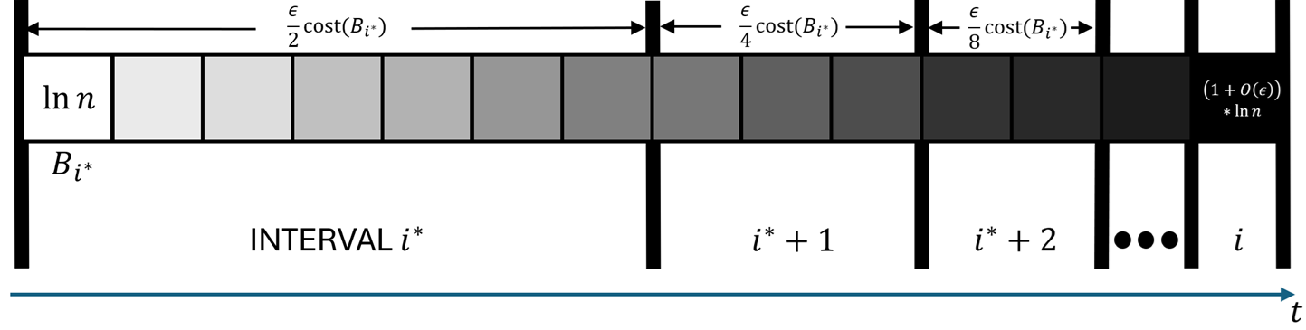
By Claim 24, we naively maintain our anchor $\mathcal{B}_{i^{*}}$ for up to $\epsilon\cdot\mathsf{cost}(\mathcal{B}_{i^{*}})$ update steps, so we can apply Lemma 16 on it with $\delta=\epsilon$ and conclude with the following corollary:

Corollary 25.

The naively maintained anchor is a $((1+O(\epsilon))\cdot\ln n)$ -approximate SC throughout the $i$ -th interval.

Observation 26.

The cost of the target solution is bounded by $(1+O(\epsilon))\cdot\mathsf{cost}(\mathcal{B}_{i^{*}})$ .

Proof.

We have that:

\mathsf{cost}(\mathcal{B}_{i}\cup\mathcal{N}_{i})\leq\mathsf{cost}(\mathcal{B}% _{i})+\mathsf{cost}(\mathcal{N}_{i})<\mathsf{cost}(\mathcal{X}_{i})+\frac{% \epsilon}{6}\mathsf{cost}(\mathcal{X}_{i})=\left(1+\frac{\epsilon}{6}\right)% \mathsf{cost}(\mathcal{X}_{i}).

Setting $j=i$ in Claim 23 yields:

\mathsf{cost}(\mathcal{B}_{i}\cup\mathcal{N}_{i})<\left(1+\frac{\epsilon}{6}% \right)\left(1+\frac{\epsilon}{2}\right)\cdot\mathsf{cost}(\mathcal{B}_{i^{*}}),

and so the claim holds. $\hfill\blacktriangleleft$ Setting $j=i$ in Claim 23 also immediately yields the following observation:

Observation 27.

The cost of the source solution is bounded by $(1+O(\epsilon))\cdot\mathsf{cost}(\mathcal{B}_{i^{*}})$ .

Throughout the $i$ -th interval our output solution is contained in $(\mathcal{B}_{i}\cup\mathcal{N}_{i}\cup\mathcal{X}_{i})$ . Since $\mathsf{cost}(\mathcal{B}_{i}\cup\mathcal{N}_{i}\cup\mathcal{X}_{i})\leq% \mathsf{cost}(\mathcal{B}_{i}\cup\mathcal{N}_{i})+\mathsf{cost}(\mathcal{X}_{i})$ , the following corollary follows directly from Corollary 25, Observation 26 and Observation 27:

Corollary 28.

If $\mathsf{cost}(\mathcal{X}_{i})>\mathsf{cost}(\mathcal{B}_{i})$ , then throughout the $i$ -th interval the output solution gives an approximation ratio of $(2+O(\epsilon))\cdot\ln n$ .

By combining Corollary 22 and Corollary 28, we obtain the following:

Corollary 29.

Throughout the entire update sequence, the output solution achieves an approximation ratio of $(2+O(\epsilon))\cdot\ln n$ .

The proof of Theorem 3 follows from Observation 19, Observation 20, Observation 21 and Corollary 29, after appropriately scaling $\epsilon$ .

5 Conclusions and Open Questions

We presented a simple black-box transformation that takes any dynamic set cover (SC) algorithm $\mathcal{ALG}$ and produces a dynamic SC algorithm with similar approximation and update time guarantees, while ensuring a worst-case recourse of $O(\alpha\cdot C)$ , where $\alpha$ is the approximation factor of $\mathcal{ALG}$ and $C$ is the aspect ratio. This transformation comes with three limitations: (1) the approximation factor increases by roughly a factor of two; (2) the recourse depends linearly on $C$ ; and (3) the recourse depends linearly on $\alpha$ .

To address limitation (3), we identified a robustness property of the classic greedy algorithm – which does not hold for primal–dual (PD) algorithms – and showed that the greedy-based dynamic algorithm of [41] maintains a robust SC at all times. By leveraging this property in a nontrivial way, we removed the $\alpha=\ln n$ dependence in the recourse bound for the high-frequency regime, improving it from $O(\log n\cdot C)$ to $O(C)$ . In contrast, in the low-frequency regime, we showed that removing the $\alpha=f$ dependence is impossible when relying on PD-based algorithms.

Our black-box transformation relies on the reconfiguration problem. As discussed in Section 2.1, even for vertex cover this framework inherently incurs the approximation blow-up in (1), as well as the recourse dependencies in (2) and (3).

This leaves the following open question. Is there an alternative approach – possibly abandoning the black-box paradigm – that avoids limitations (1) and (2)? In particular, can one reduce or eliminate the factor- $2$ loss in the approximation guarantee and/or achieve a sublinear, preferably polylogarithmic, dependence on the aspect ratio $C$ ? We view these as the main directions for future work.

References

[1] Amir Abboud, Raghavendra Addanki, Fabrizio Grandoni, Debmalya Panigrahi, and Barna Saha. Dynamic set cover: improved algorithms and lower bounds. In Proceedings of the 51st Annual ACM SIGACT Symposium on Theory of Computing, pages 114–125, 2019. doi:10.1145/3313276.3316376.
[2] Spyros Angelopoulos, Christoph Dürr, and Shendan Jin. Online maximum matching with recourse. J. Comb. Optim., 40(4):974–1007, 2020. doi:10.1007/s10878-020-00641-w.
[3] Sepehr Assadi, Krzysztof Onak, Baruch Schieber, and Shay Solomon. Fully dynamic maximal independent set with sublinear update time. In Proceedings of the 50th Annual ACM SIGACT Symposium on Theory of Computing, STOC 2018, pages 815–826, New York, NY, USA, 2018. Association for Computing Machinery. doi:10.1145/3188745.3188922.
[4] Sepehr Assadi and Shay Solomon. Fully Dynamic Set Cover via Hypergraph Maximal Matching: An Optimal Approximation Through a Local Approach. In 29th Annual European Symposium on Algorithms (ESA 2021), volume 204 of Leibniz International Proceedings in Informatics (LIPIcs), pages 8:1–8:18. Schloss Dagstuhl – Leibniz-Zentrum für Informatik, 2021. doi:10.4230/LIPIcs.ESA.2021.8.
[5] Nikhil Bansal, Anupam Gupta, Ravishankar Krishnaswamy, Kirk Pruhs, Kevin Schewior, and Cliff Stein. A 2-Competitive Algorithm For Online Convex Optimization With Switching Costs. In Naveen Garg, Klaus Jansen, Anup Rao, and José D. P. Rolim, editors, Approximation, Randomization, and Combinatorial Optimization. Algorithms and Techniques (APPROX/RANDOM 2015), volume 40 of Leibniz International Proceedings in Informatics (LIPIcs), pages 96–109, Dagstuhl, Germany, 2015. Schloss Dagstuhl – Leibniz-Zentrum für Informatik. doi:10.4230/LIPIcs.APPROX-RANDOM.2015.96.
[6] Surender Baswana, Manoj Gupta, and Sandeep Sen. Fully dynamic maximal matching in O(logn) update time. In 2011 IEEE 52nd Annual Symposium on Foundations of Computer Science, pages 383–392, 2011. doi:10.1109/FOCS.2011.89.
[7] Soheil Behnezhad, Mahsa Derakhshan, MohammadTaghi Hajiaghayi, Cliff Stein, and Madhu Sudan. Fully dynamic maximal independent set with polylogarithmic update time. In 2019 IEEE 60th Annual Symposium on Foundations of Computer Science (FOCS), pages 382–405, 2019. doi:10.1109/FOCS.2019.00032.
[8] Aaron Bernstein, Jacob Holm, and Eva Rotenberg. Online bipartite matching with amortized O $(\log^{2}n)$ replacements. J. ACM, 66(5), 2019. doi:10.1145/3344999.
[9] Aaron Bernstein, Tsvi Kopelowitz, Seth Pettie, Ely Porat, and Clifford Stein. Simultaneously Load Balancing for Every p-norm, With Reassignments. In Christos H. Papadimitriou, editor, 8th Innovations in Theoretical Computer Science Conference (ITCS 2017), volume 67 of Leibniz International Proceedings in Informatics (LIPIcs), pages 51:1–51:14, Dagstuhl, Germany, 2017. Schloss Dagstuhl – Leibniz-Zentrum für Informatik. doi:10.4230/LIPIcs.ITCS.2017.51.
[10] Sayan Bhattacharya, Ruoxu Cen, and Debmalya Panigrahi. Fully dynamic set cover: Worst-case recourse and update time. CoRR, abs/2511.08485, November 2025. Accepted to STOC 2026. doi:10.48550/arXiv.2511.08485.
[11] Sayan Bhattacharya, Deeparnab Chakrabarty, and Monika Henzinger. Deterministic fully dynamic approximate vertex cover and fractional matching in O(1) amortized update time. In International Conference on Integer Programming and Combinatorial Optimization, pages 86–98. Springer, 2017. doi:10.1007/978-3-319-59250-3_8.
[12] Sayan Bhattacharya, Monika Henzinger, and Giuseppe F Italiano. Design of dynamic algorithms via primal-dual method. In International Colloquium on Automata, Languages, and Programming, pages 206–218. Springer, 2015. doi:10.1007/978-3-662-47672-7_17.
[13] Sayan Bhattacharya, Monika Henzinger, and Danupon Nanongkai. A new deterministic algorithm for dynamic set cover. In 2019 IEEE 60th Annual Symposium on Foundations of Computer Science (FOCS), pages 406–423. IEEE, 2019. doi:10.1109/FOCS.2019.00033.
[14] Sayan Bhattacharya, Monika Henzinger, Danupon Nanongkai, and Xiaowei Wu. Dynamic set cover: Improved amortized and worst-case update time. In Proceedings of the 2021 ACM-SIAM Symposium on Discrete Algorithms (SODA), pages 2537–2549. SIAM, 2021. doi:10.1137/1.9781611976465.150.
[15] Sayan Bhattacharya and Janardhan Kulkarni. Deterministically Maintaining a $(2+\epsilon)$ -Approximate Minimum Vertex Cover in O $(1/\epsilon^{2})$ Amortized Update Time, pages 1872–1885. SIAM, January 2019. doi:10.1137/1.9781611975482.113.
[16] Bartłomiej Bosek, Dariusz Leniowski, Piotr Sankowski, and Anna Zych. A Tight Bound for Shortest Augmenting Paths on Trees, pages 201–216. Springer, March 2018. doi:10.1007/978-3-319-77404-6_16.
[17] Anton Bukov, Shay Solomon, and Tianyi Zhang. Nearly optimal dynamic set cover: Breaking the quadratic-in- $f$ time barrier. arXiv preprint arXiv:2308.00793, 2023. doi:10.48550/arXiv.2308.00793.
[18] Keren Censor-Hillel, Elad Haramaty, and Zohar Karnin. Optimal dynamic distributed mis. In Proceedings of the 2016 ACM Symposium on Principles of Distributed Computing, PODC ’16, pages 217–226, New York, NY, USA, 2016. Association for Computing Machinery. doi:10.1145/2933057.2933083.
[19] K. Chaudhuri, C. Daskalakis, R. D. Kleinberg, and H. Lin. Online bipartite perfect matching with augmentations. In IEEE INFOCOM 2009, pages 1044–1052, 2009. doi:10.1109/INFCOM.2009.5062016.
[20] Shiri Chechik and Tianyi Zhang. Fully dynamic maximal independent set in expected poly-log update time. In 2019 IEEE 60th Annual Symposium on Foundations of Computer Science (FOCS), pages 370–381, 2019. doi:10.1109/FOCS.2019.00031.
[21] Irit Dinur and David Steurer. Analytical approach to parallel repetition. In Proceedings of the forty-sixth annual ACM symposium on Theory of computing, pages 624–633, 2014. doi:10.1145/2591796.2591884.
[22] Edward F. Grove, Ming-Yang Kao, P. Krishnan, and Jeffrey Scott Vitter. Online perfect matching and mobile computing. In Proceedings of the 4th International Workshop on Algorithms and Data Structures, WADS ’95, pages 194–205, Berlin, Heidelberg, 1995. Springer-Verlag. doi:10.1007/3-540-60220-8_62.
[23] Albert Gu, Anupam Gupta, and Amit Kumar. The power of deferral: maintaining a constant-competitive steiner tree online. In Proceedings of the Forty-Fifth Annual ACM Symposium on Theory of Computing, STOC ’13, pages 525–534, New York, NY, USA, 2013. Association for Computing Machinery. doi:10.1145/2488608.2488674.
[24] Anupam Gupta, Ravishankar Krishnaswamy, Amit Kumar, and Debmalya Panigrahi. Online and dynamic algorithms for set cover. In Proceedings of the 49th Annual ACM SIGACT Symposium on Theory of Computing, pages 537–550, 2017. doi:10.1145/3055399.3055493.
[25] Anupam Gupta and Amit Kumar. Online steiner tree with deletions. In Proceedings of the Twenty-Fifth Annual ACM-SIAM Symposium on Discrete Algorithms, SODA ’14, pages 455–467, USA, 2014. Society for Industrial and Applied Mathematics. doi:10.1137/1.9781611973402.34.
[26] Anupam Gupta, Amit Kumar, and Cliff Stein. Maintaining Assignments Online: Matching, Scheduling, and Flows, pages 468–479. SIAM, 2014. doi:10.1137/1.9781611973402.35.
[27] Manoj Gupta and Richard Peng. Fully Dynamic $(1+\epsilon)$ -Approximate Matchings . In 2013 IEEE 54th Annual Symposium on Foundations of Computer Science (FOCS), pages 548–557, Los Alamitos, CA, USA, October 2013. IEEE Computer Society. doi:10.1109/FOCS.2013.65.
[28] Jan van den Heuvel. The complexity of change, pages 127–160. London Mathematical Society Lecture Note Series. Cambridge University Press, 2013. doi:10.1017/CBO9781139506748.005.
[29] Niklas Hjuler, Giuseppe F. Italiano, Nikos Parotsidis, and David Saulpic. Dominating Sets and Connected Dominating Sets in Dynamic Graphs. In Rolf Niedermeier and Christophe Paul, editors, 36th International Symposium on Theoretical Aspects of Computer Science (STACS 2019), volume 126 of Leibniz International Proceedings in Informatics (LIPIcs), pages 35:1–35:17, Dagstuhl, Germany, 2019. Schloss Dagstuhl – Leibniz-Zentrum für Informatik. doi:10.4230/LIPIcs.STACS.2019.35.
[30] Takehiro Ito, Erik D. Demaine, Nicholas J. A. Harvey, Christos H. Papadimitriou, Martha Sideri, Ryuhei Uehara, and Yushi Uno. On the complexity of reconfiguration problems. Theor. Comput. Sci., 412(12–14):1054–1065, 2011. doi:10.1016/j.tcs.2010.12.005.
[31] Subhash Khot and Oded Regev. Vertex cover might be hard to approximate to within $2-\varepsilon$ . Journal of Computer and System Sciences, 74(3):335–349, 2008.
[32] Nicole Megow, Martin Skutella, José Verschae, and Andreas Wiese. The power of recourse for online mst and tsp. SIAM Journal on Computing, 45(3):859–880, 2016. doi:10.1137/130917703.
[33] Ofer Neiman and Shay Solomon. Simple deterministic algorithms for fully dynamic maximal matching. ACM Trans. Algorithms, 12(1), 2015. doi:10.1145/2700206.
[34] Naomi Nishimura. Introduction to reconfiguration. Algorithms, 11(4), 2018. doi:10.3390/a11040052.
[35] Krzysztof Onak and Ronitt Rubinfeld. Maintaining a large matching and a small vertex cover. In Proceedings of the Forty-Second ACM Symposium on Theory of Computing, STOC ’10, pages 457–464, New York, NY, USA, 2010. Association for Computing Machinery. doi:10.1145/1806689.1806753.
[36] David Peleg and Shay Solomon. Dynamic $(1+\epsilon)$ -Approximate Matchings: A Density-Sensitive Approach, pages 712–729. SIAM, 2016. doi:10.1137/1.9781611974331.ch51.
[37] Noam Solomon and Shay Solomon. A Generalized Matching Reconfiguration Problem. In James R. Lee, editor, 12th Innovations in Theoretical Computer Science Conference (ITCS 2021), volume 185 of Leibniz International Proceedings in Informatics (LIPIcs), pages 57:1–57:20, Dagstuhl, Germany, 2021. Schloss Dagstuhl – Leibniz-Zentrum für Informatik. doi:10.4230/LIPIcs.ITCS.2021.57.
[38] Shay Solomon. Fully Dynamic Maximal Matching in Constant Update Time . In 2016 IEEE 57th Annual Symposium on Foundations of Computer Science (FOCS), pages 325–334, Los Alamitos, CA, USA, October 2016. IEEE Computer Society. doi:10.1109/FOCS.2016.43.
[39] Shay Solomon. Local algorithms for bounded degree sparsifiers in sparse graphs. In Anna R. Karlin, editor, 9th Innovations in Theoretical Computer Science Conference, ITCS 2018, January 11-14, 2018, Cambridge, MA, USA, volume 94 of LIPIcs, pages 52:1–52:19. Schloss Dagstuhl – Leibniz-Zentrum für Informatik, 2018. doi:10.4230/LIPIcs.ITCS.2018.52.
[40] Shay Solomon and Amitai Uzrad. Dynamic $((1+\epsilon)\ln n)$ -Approximation Algorithms for Minimum Set Cover and Dominating Set. In Proceedings of the 55th Annual ACM Symposium on Theory of Computing, pages 1187–1200, 2023. doi:10.1145/3564246.3585211.
[41] Shay Solomon, Amitai Uzrad, and Tianyi Zhang. A lossless deamortization for dynamic greedy set cover. In 2024 IEEE 65th Annual Symposium on Foundations of Computer Science (FOCS), pages 264–290, 2024. doi:10.1109/FOCS61266.2024.00025.
[42] David P Williamson and David B Shmoys. The design of approximation algorithms. Cambridge university press, 2011.

[bib.bib1] [1] Amir Abboud, Raghavendra Addanki, Fabrizio Grandoni, Debmalya Panigrahi, and Barna Saha. Dynamic set cover: improved algorithms and lower bounds. In Proceedings of the 51st Annual ACM SIGACT Symposium on Theory of Computing, pages 114–125, 2019. doi:10.1145/3313276.3316376.

[bib.bib2] [2] Spyros Angelopoulos, Christoph Dürr, and Shendan Jin. Online maximum matching with recourse. J. Comb. Optim., 40(4):974–1007, 2020. doi:10.1007/s10878-020-00641-w.

[bib.bib3] [3] Sepehr Assadi, Krzysztof Onak, Baruch Schieber, and Shay Solomon. Fully dynamic maximal independent set with sublinear update time. In Proceedings of the 50th Annual ACM SIGACT Symposium on Theory of Computing, STOC 2018, pages 815–826, New York, NY, USA, 2018. Association for Computing Machinery. doi:10.1145/3188745.3188922.

[bib.bib4] [4] Sepehr Assadi and Shay Solomon. Fully Dynamic Set Cover via Hypergraph Maximal Matching: An Optimal Approximation Through a Local Approach. In 29th Annual European Symposium on Algorithms (ESA 2021), volume 204 of Leibniz International Proceedings in Informatics (LIPIcs), pages 8:1–8:18. Schloss Dagstuhl – Leibniz-Zentrum für Informatik, 2021. doi:10.4230/LIPIcs.ESA.2021.8.

[bib.bib5] [5] Nikhil Bansal, Anupam Gupta, Ravishankar Krishnaswamy, Kirk Pruhs, Kevin Schewior, and Cliff Stein. A 2-Competitive Algorithm For Online Convex Optimization With Switching Costs. In Naveen Garg, Klaus Jansen, Anup Rao, and José D. P. Rolim, editors, Approximation, Randomization, and Combinatorial Optimization. Algorithms and Techniques (APPROX/RANDOM 2015), volume 40 of Leibniz International Proceedings in Informatics (LIPIcs), pages 96–109, Dagstuhl, Germany, 2015. Schloss Dagstuhl – Leibniz-Zentrum für Informatik. doi:10.4230/LIPIcs.APPROX-RANDOM.2015.96.

[bib.bib6] [6] Surender Baswana, Manoj Gupta, and Sandeep Sen. Fully dynamic maximal matching in O(logn) update time. In 2011 IEEE 52nd Annual Symposium on Foundations of Computer Science, pages 383–392, 2011. doi:10.1109/FOCS.2011.89.

[bib.bib7] [7] Soheil Behnezhad, Mahsa Derakhshan, MohammadTaghi Hajiaghayi, Cliff Stein, and Madhu Sudan. Fully dynamic maximal independent set with polylogarithmic update time. In 2019 IEEE 60th Annual Symposium on Foundations of Computer Science (FOCS), pages 382–405, 2019. doi:10.1109/FOCS.2019.00032.

[bib.bib8] [8] Aaron Bernstein, Jacob Holm, and Eva Rotenberg. Online bipartite matching with amortized O $(\log^{2}n)$ replacements. J. ACM, 66(5), 2019. doi:10.1145/3344999.

[bib.bib9] [9] Aaron Bernstein, Tsvi Kopelowitz, Seth Pettie, Ely Porat, and Clifford Stein. Simultaneously Load Balancing for Every p-norm, With Reassignments. In Christos H. Papadimitriou, editor, 8th Innovations in Theoretical Computer Science Conference (ITCS 2017), volume 67 of Leibniz International Proceedings in Informatics (LIPIcs), pages 51:1–51:14, Dagstuhl, Germany, 2017. Schloss Dagstuhl – Leibniz-Zentrum für Informatik. doi:10.4230/LIPIcs.ITCS.2017.51.

[bib.bib10] [10] Sayan Bhattacharya, Ruoxu Cen, and Debmalya Panigrahi. Fully dynamic set cover: Worst-case recourse and update time. CoRR, abs/2511.08485, November 2025. Accepted to STOC 2026. doi:10.48550/arXiv.2511.08485.

[bib.bib11] [11] Sayan Bhattacharya, Deeparnab Chakrabarty, and Monika Henzinger. Deterministic fully dynamic approximate vertex cover and fractional matching in O(1) amortized update time. In International Conference on Integer Programming and Combinatorial Optimization, pages 86–98. Springer, 2017. doi:10.1007/978-3-319-59250-3_8.

[bib.bib12] [12] Sayan Bhattacharya, Monika Henzinger, and Giuseppe F Italiano. Design of dynamic algorithms via primal-dual method. In International Colloquium on Automata, Languages, and Programming, pages 206–218. Springer, 2015. doi:10.1007/978-3-662-47672-7_17.

[bib.bib13] [13] Sayan Bhattacharya, Monika Henzinger, and Danupon Nanongkai. A new deterministic algorithm for dynamic set cover. In 2019 IEEE 60th Annual Symposium on Foundations of Computer Science (FOCS), pages 406–423. IEEE, 2019. doi:10.1109/FOCS.2019.00033.

[bib.bib14] [14] Sayan Bhattacharya, Monika Henzinger, Danupon Nanongkai, and Xiaowei Wu. Dynamic set cover: Improved amortized and worst-case update time. In Proceedings of the 2021 ACM-SIAM Symposium on Discrete Algorithms (SODA), pages 2537–2549. SIAM, 2021. doi:10.1137/1.9781611976465.150.

[bib.bib15] [15] Sayan Bhattacharya and Janardhan Kulkarni. Deterministically Maintaining a $(2+\epsilon)$ -Approximate Minimum Vertex Cover in O $(1/\epsilon^{2})$ Amortized Update Time, pages 1872–1885. SIAM, January 2019. doi:10.1137/1.9781611975482.113.

[bib.bib16] [16] Bartłomiej Bosek, Dariusz Leniowski, Piotr Sankowski, and Anna Zych. A Tight Bound for Shortest Augmenting Paths on Trees, pages 201–216. Springer, March 2018. doi:10.1007/978-3-319-77404-6_16.

[bib.bib17] [17] Anton Bukov, Shay Solomon, and Tianyi Zhang. Nearly optimal dynamic set cover: Breaking the quadratic-in- $f$ time barrier. arXiv preprint arXiv:2308.00793, 2023. doi:10.48550/arXiv.2308.00793.

[bib.bib18] [18] Keren Censor-Hillel, Elad Haramaty, and Zohar Karnin. Optimal dynamic distributed mis. In Proceedings of the 2016 ACM Symposium on Principles of Distributed Computing, PODC ’16, pages 217–226, New York, NY, USA, 2016. Association for Computing Machinery. doi:10.1145/2933057.2933083.

[bib.bib19] [19] K. Chaudhuri, C. Daskalakis, R. D. Kleinberg, and H. Lin. Online bipartite perfect matching with augmentations. In IEEE INFOCOM 2009, pages 1044–1052, 2009. doi:10.1109/INFCOM.2009.5062016.

[bib.bib20] [20] Shiri Chechik and Tianyi Zhang. Fully dynamic maximal independent set in expected poly-log update time. In 2019 IEEE 60th Annual Symposium on Foundations of Computer Science (FOCS), pages 370–381, 2019. doi:10.1109/FOCS.2019.00031.

[bib.bib21] [21] Irit Dinur and David Steurer. Analytical approach to parallel repetition. In Proceedings of the forty-sixth annual ACM symposium on Theory of computing, pages 624–633, 2014. doi:10.1145/2591796.2591884.

[bib.bib22] [22] Edward F. Grove, Ming-Yang Kao, P. Krishnan, and Jeffrey Scott Vitter. Online perfect matching and mobile computing. In Proceedings of the 4th International Workshop on Algorithms and Data Structures, WADS ’95, pages 194–205, Berlin, Heidelberg, 1995. Springer-Verlag. doi:10.1007/3-540-60220-8_62.

[bib.bib23] [23] Albert Gu, Anupam Gupta, and Amit Kumar. The power of deferral: maintaining a constant-competitive steiner tree online. In Proceedings of the Forty-Fifth Annual ACM Symposium on Theory of Computing, STOC ’13, pages 525–534, New York, NY, USA, 2013. Association for Computing Machinery. doi:10.1145/2488608.2488674.

[bib.bib24] [24] Anupam Gupta, Ravishankar Krishnaswamy, Amit Kumar, and Debmalya Panigrahi. Online and dynamic algorithms for set cover. In Proceedings of the 49th Annual ACM SIGACT Symposium on Theory of Computing, pages 537–550, 2017. doi:10.1145/3055399.3055493.

[bib.bib25] [25] Anupam Gupta and Amit Kumar. Online steiner tree with deletions. In Proceedings of the Twenty-Fifth Annual ACM-SIAM Symposium on Discrete Algorithms, SODA ’14, pages 455–467, USA, 2014. Society for Industrial and Applied Mathematics. doi:10.1137/1.9781611973402.34.

[bib.bib26] [26] Anupam Gupta, Amit Kumar, and Cliff Stein. Maintaining Assignments Online: Matching, Scheduling, and Flows, pages 468–479. SIAM, 2014. doi:10.1137/1.9781611973402.35.

[bib.bib27] [27] Manoj Gupta and Richard Peng. Fully Dynamic $(1+\epsilon)$ -Approximate Matchings . In 2013 IEEE 54th Annual Symposium on Foundations of Computer Science (FOCS), pages 548–557, Los Alamitos, CA, USA, October 2013. IEEE Computer Society. doi:10.1109/FOCS.2013.65.

[bib.bib28] [28] Jan van den Heuvel. The complexity of change, pages 127–160. London Mathematical Society Lecture Note Series. Cambridge University Press, 2013. doi:10.1017/CBO9781139506748.005.

[bib.bib29] [29] Niklas Hjuler, Giuseppe F. Italiano, Nikos Parotsidis, and David Saulpic. Dominating Sets and Connected Dominating Sets in Dynamic Graphs. In Rolf Niedermeier and Christophe Paul, editors, 36th International Symposium on Theoretical Aspects of Computer Science (STACS 2019), volume 126 of Leibniz International Proceedings in Informatics (LIPIcs), pages 35:1–35:17, Dagstuhl, Germany, 2019. Schloss Dagstuhl – Leibniz-Zentrum für Informatik. doi:10.4230/LIPIcs.STACS.2019.35.

[bib.bib30] [30] Takehiro Ito, Erik D. Demaine, Nicholas J. A. Harvey, Christos H. Papadimitriou, Martha Sideri, Ryuhei Uehara, and Yushi Uno. On the complexity of reconfiguration problems. Theor. Comput. Sci., 412(12–14):1054–1065, 2011. doi:10.1016/j.tcs.2010.12.005.

[bib.bib31] [31] Subhash Khot and Oded Regev. Vertex cover might be hard to approximate to within $2-\varepsilon$ . Journal of Computer and System Sciences, 74(3):335–349, 2008.

[bib.bib32] [32] Nicole Megow, Martin Skutella, José Verschae, and Andreas Wiese. The power of recourse for online mst and tsp. SIAM Journal on Computing, 45(3):859–880, 2016. doi:10.1137/130917703.

[bib.bib33] [33] Ofer Neiman and Shay Solomon. Simple deterministic algorithms for fully dynamic maximal matching. ACM Trans. Algorithms, 12(1), 2015. doi:10.1145/2700206.

[bib.bib34] [34] Naomi Nishimura. Introduction to reconfiguration. Algorithms, 11(4), 2018. doi:10.3390/a11040052.

[bib.bib35] [35] Krzysztof Onak and Ronitt Rubinfeld. Maintaining a large matching and a small vertex cover. In Proceedings of the Forty-Second ACM Symposium on Theory of Computing, STOC ’10, pages 457–464, New York, NY, USA, 2010. Association for Computing Machinery. doi:10.1145/1806689.1806753.

[bib.bib36] [36] David Peleg and Shay Solomon. Dynamic $(1+\epsilon)$ -Approximate Matchings: A Density-Sensitive Approach, pages 712–729. SIAM, 2016. doi:10.1137/1.9781611974331.ch51.

[bib.bib37] [37] Noam Solomon and Shay Solomon. A Generalized Matching Reconfiguration Problem. In James R. Lee, editor, 12th Innovations in Theoretical Computer Science Conference (ITCS 2021), volume 185 of Leibniz International Proceedings in Informatics (LIPIcs), pages 57:1–57:20, Dagstuhl, Germany, 2021. Schloss Dagstuhl – Leibniz-Zentrum für Informatik. doi:10.4230/LIPIcs.ITCS.2021.57.

[bib.bib38] [38] Shay Solomon. Fully Dynamic Maximal Matching in Constant Update Time . In 2016 IEEE 57th Annual Symposium on Foundations of Computer Science (FOCS), pages 325–334, Los Alamitos, CA, USA, October 2016. IEEE Computer Society. doi:10.1109/FOCS.2016.43.

[bib.bib39] [39] Shay Solomon. Local algorithms for bounded degree sparsifiers in sparse graphs. In Anna R. Karlin, editor, 9th Innovations in Theoretical Computer Science Conference, ITCS 2018, January 11-14, 2018, Cambridge, MA, USA, volume 94 of LIPIcs, pages 52:1–52:19. Schloss Dagstuhl – Leibniz-Zentrum für Informatik, 2018. doi:10.4230/LIPIcs.ITCS.2018.52.

[bib.bib40] [40] Shay Solomon and Amitai Uzrad. Dynamic $((1+\epsilon)\ln n)$ -Approximation Algorithms for Minimum Set Cover and Dominating Set. In Proceedings of the 55th Annual ACM Symposium on Theory of Computing, pages 1187–1200, 2023. doi:10.1145/3564246.3585211.

[bib.bib41] [41] Shay Solomon, Amitai Uzrad, and Tianyi Zhang. A lossless deamortization for dynamic greedy set cover. In 2024 IEEE 65th Annual Symposium on Foundations of Computer Science (FOCS), pages 264–290, 2024. doi:10.1109/FOCS61266.2024.00025.

[bib.bib42] [42] David P Williamson and David B Shmoys. The design of approximation algorithms. Cambridge university press, 2011.

Dynamic Set Cover with Worst-Case Recourse

Abstract

Keywords and phrases:

Category:

Funding:

Copyright and License:

2012 ACM Subject Classification:

DOI:

Event:

Editors:

Series and Publisher:

1 Introduction

Dynamic Set Cover.

Recourse.

Amortized Versus Worst-case.

Our Focus.

1.1 Prior Work

Slow Update Time, Worst-Case Recourse.

Slow Update Time, Amortized Recourse.

Fast Amortized Time, Amortized Recourse.

Fast Worst-case Time, High Recourse.

Question 1.

1.2 Our Contribution

Theorem 1 (Black-box Transformation).

Corollary 2 (Low-Frequency).

Remarks.

Theorem 3 (High-Frequency).

Remark.

Theorem 4 (Dominating Set).

1.3 Concurrent Work

1.4 Organization

2 𝑶⁢(𝜶⁢𝑪ϵ) Worst-case Recourse: Black-box Transformation

2.1 A Static Reconfiguration Problem

2.2 Overview

2.3 Algorithm

2.4 Analysis

Observation 5 (Recourse).

Proof.

Observation 6 (Update Time).

Proof.

Observation 7 (Legal Solution).

Proof.

Claim 8 (Approximation Factor).

2.4.1 Proof of Claim 8

Observation 9.

Observation 10.

Proof.

Observation 11.

Proof.

Observation 12.

Proof.

Observation 13.

Proof.

3 The Robustness Property

3.1 The Robustness Property I: The Greedy and PD Static Algorithms

Observation 14 (Warm-up: Static greedy is robust).

Proof.

Claim 15.

Proof.

Remark.

The classic PD algorithm is not robust.

3.2 The Robustness Property II: The Dynamic Algorithm [41]

Lemma 16 ([41] is Robust - Greedy-Based).

3.2.1 Preliminaries

Definition 17.

3.2.2 Invariants

3.2.3 Proof of Lemma 16

Part I – Similar to [41].

Part II – New Ideas.

Part III – Similar to [41].

4 Worst-Case Recourse: 𝑶⁢(𝐥𝐨𝐠⁡𝒏⋅𝑪ϵ) to 𝑶⁢(𝑪ϵ) (Greedy)

Theorem 18 ([41] – Greedy-Based).

4.1 Algorithm Description

Observation 19 (Recourse).

Proof.

Observation 20 (Update Time).

Proof.

Observation 21 (Legal Solution).

Proof.

4.2 Approximation Factor

2 $O\left(\frac{\alpha C}{\epsilon}\right)$ Worst-case Recourse: Black-box Transformation

4 Worst-Case Recourse: $O\left(\frac{\log n\cdot C}{\epsilon}\right)$ to $O\left(\frac{C}{\epsilon}\right)$ (Greedy)