Online Metric TSP: Beyond the Barrier

Abstract
We study an online variant of the Traveling Salesperson Problem (TSP) in which points arrive sequentially and must be inserted into an evolving tour. In the classical setting where arbitrary insertions are allowed, an -competitive algorithm has been known since the 1970s (Rosenkrantz, Stearns and Lewis 1977, Imase and Waxman 1991). Recently, Abrahamsen, Bercea, Beretta, Klausen, and Kozma [ESA 2024] introduced online metric TSP, a stricter model in which each arriving point must be assigned to a distinct cell of an array of size , with the final tour order induced by the non-empty cells; the parameter captures the space usage of the algorithm.
When , this model recovers arbitrary insertions and therefore admits an -competitive algorithm. In contrast, when , i.e., when each point’s position is fixed on arrival, Bertram [7] recently showed that the competitive ratio is . We investigate the tradeoff between space usage and competitiveness between these extremes. We note that this tradeoff was previously explored by the authors in [6] for the online sorting problem, which is the special case of online metric TSP on a line metric.
Our main result is a deterministic online metric TSP algorithm using space that achieves a competitive ratio of , for any . In particular, increasing the space from to improves the competitive ratio from to . We complement this with a lower bound showing that for , any deterministic algorithm has a competitive ratio , for all . Consequently, even with , deterministic algorithms cannot achieve a constant competitive ratio.
Keywords and phrases:
Online algorithms, competitive analysis, metric TSP, space-competitiveness tradeoff, routing problemsCategory:
Track A: Algorithms, Complexity and GamesFunding:
Debmalya Panigrahi: D. Panigrahi was supported in part by NSF grants CCF-1955703 and CCF-2329230.Copyright and License:
![[Uncaptioned image]](x1.png) © Yossi Azar, Debmalya Panigrahi, and Or Vardi; licensed under Creative Commons License CC-BY 4.0
© Yossi Azar, Debmalya Panigrahi, and Or Vardi; licensed under Creative Commons License CC-BY 4.0
2012 ACM Subject Classification:
Theory of computation Online algorithms ; Theory of computation Routing and network design problems ; Theory of computation Approximation algorithms analysisEditors:
Sayan Bhattacharya, Danupon Nanongkai, Michael Benedikt, and Gabriele PuppisSeries and Publisher:
 Leibniz International Proceedings in Informatics, Schloss Dagstuhl – Leibniz-Zentrum für Informatik
1 Introduction
The (metric) traveling salesman problem (TSP) is a classic problem in combinatorial optimization where the goal is to find the minimum-length tour covering a set of points in a metric space. In a classic result in approximation algorithms, Christofides [10] (and independently, Serdyukov [25]) gave a -approximation to this problem, which remained the state-of-the-art for almost 50 years before being eventually improved to (for a small ) in a remarkable recent result of Karlin, Klein, and Oveis Gharan [16]. On the hardness side, Papadimitrou and Yannakakis [23] showed APX-hardness for this problem as a consequence of the PCP theorem [3]; the current record on the lower bound stands at [17]. Resolving this gap remains a central open question in approximation algorithms.
What if the set of points that we need to connect is not known in advance but arrives online? In each online step, the goal is to insert the newly arriving point in the existing order in a way that minimizes the length of the tour following that order. In the classical version of this problem, where the arriving point can be inserted anywhere in the existing order, -competitive algorithms are known since the 1970s [24, 14]. Recently, Abrahamsen, Bercea, Beretta, Klausen, and Kozma [2] introduced a stricter model called online metric TSP: here, the online algorithm has to map each arriving point to a distinct cell of an array of size , and the eventual order is given by the sequence of non-empty cells in the array. (We refer to the parameter as the space usage of the algorithm.) If , this setting recovers arbitrary insertions thereby admitting a competitive ratio of . At the other extreme, when , the online algorithm commits to an irrevocable position of the new point in the eventual order immediately on arrival. For this setting, Bertram [7] recently gave a deterministic algorithm with a competitive ratio of , matching previously known lower bounds even allowing randomization [1, 2]. The exponential gap in the competitive ratio between the two extremes raises a natural question about what lies in between, namely: how does the competitive ratio of online metric TSP depend on the space usage ?
We note that this tradeoff between competitive ratio and space usage was previously explored by the authors for the online sorting problem [6] introduced by Aamand, Abrahamsen, Beretta, and Kleist [1], which is the special case of online metric TSP on a line metric. We will describe later that the solution proposed by [6] for online sorting does not generalize naturally to online metric TSP; indeed, the algorithm given in this paper is a different, and arguably more natural, solution for the online sorting problem as well. Moreover, the lower bound in this paper is applicable to the online sorting problem as well. Therefore, in addition to studying online metric TSP with , this paper makes contributions to the online sorting problem for the case of as well.
1.1 Our Results
In this paper, we answer this question by showing a poly-logarithmic competitive ratio for online metric TSP even when only mildly exceeds . Note that this is an exponential improvement over the case . Specifically, we show:
Theorem 1.
There is a deterministic online metric TSP algorithm that uses space and achieves a competitive ratio of , for any .
This implies, for instance, that with extra space, the competitive ratio of online metric TSP improves from to . Prior to our work, the only cases for which a sub-polynomial competitive ratio was known had a space usage of . It is interesting to ask whether the extra space can be reduced even further to for any constant , or whether there is a lower bound on the extra space required to obtain a competitive ratio. We leave these are interesting open questions.
Can the competitive ratio be improved further to ? To the best of our knowledge, such a result is not known even for unlimited space, but there is no lower bound either, even for . We complement our upper bound by showing that it is impossible for a deterministic algorithm to achieve a competitive ratio of , unless polynomially exceeds . We show:
Theorem 2.
For , the competitive ratio of any deterministic online metric TSP algorithm is , for any .
This implies that using even , the best competitive ratio one can potentially achieve deterministically is .
Remark.
We note that the lower bound construction that we will give later to prove Theorem 2 is actually for the online sorting problem, which is a special case of onine metric TSP. In [6], the authors showed that using , one can achieve a competitive ratio of for the online sorting problem. However, this result does not contradict the lower bound in this paper since the previous result assumed that the algorithm knows the value of from the outset, while the lower bound is for the case where the value of is unknown to the algorithm. It remains open whether an -competitive algorithm exists for the online metric TSP problem for the case of known .
1.2 Related Work
Online versions of TSP have been studied since the 1970s when Rosenkrantz, Stearns, and Lewis [24] introduced the class of constructive insertion heuristics to iteratively build a TSP tour by inserting new vertices while preserving the relative order of previous vertices. They gave a -approximate algorithm when the insertion order is chosen by the algorithm, and an -competitive one when it is chosen by an adversary. The latter result also follows from later work by Imase and Waxman on the online Steiner tree problem [14], where the online algorithm additionally commits to the edges being used to connect the new vertex to the previous vertices. This latter commitment also creates a difference between the two problems: while -competitiveness is tight for online Steiner tree, it is not known to be tight for creating an online TSP tour. For the latter bound, the only lower bounds known are for specific insertion strategies, such as for the greedy strategy due to Azar [5]. (See also [21] for a recourse version of online MST and TSP where the algorithm commits to edges but these can be partially revoked using a limited budget.)
Later, a different online version of TSP was proposed, where a server has to serve a sequence of requests arriving online on a metric space and the goal is to minimize the makespan, i.e., the total time to serve all requests [4]. This problem differs from prior work (and from online metric TSP) in that there is a real notion of time with release dates for the server requests. We note that several results have been obtained in this line of work, both for general metric spaces [11, 9, 19, 18, 20, 15] and also specifically for the line metric [8].
Online metric TSP was introduced by Abrahamsen, Bercea, Beretta, Klausen, and Kozma [2] as a generalization of the online sorting problem [1] which restricts the points to a line. It is known that online sorting has a tight competitive ratio of when [1, 2], and that this bound continues to hold for online metric TSP with [7]. For , an -competitive algorithm is known for when is known, and an -competitive algorithm is known for (for ) when is unknown [6]. Note that the lower bound result in the current paper also applies to online sorting; hence, it shows that this distinction between known and unknown is necessary. Further results on the online sorting problem appear in [22, 13, 12].
1.3 Our Techniques
We now give an overview of our main techniques. We first describe our upper bound (Theorem 1) and then outline the lower bound construction (Theorem 2).
Upper Bound.
Our starting point is the previous result for the online sorting problem with [6]. This paper gave an -competitive algorithm using space, based on a novel data structure called an elementary tree. The core idea is to maintain a collection of binary trees whose leaves, ordered from left to right, correspond to array cells, and which guide the insertion of arriving elements.
We briefly recall how elementary trees are used to insert elements. The algorithm dynamically and sequentially labels internal tree nodes with dyadic intervals, whose lengths correspond to the heights of the nodes. For example, if the element range is , the root is labeled , but its two children may both be labeled , or , or one of each. This continues down the tree with the interval length halving at each level. The label of a node specifies the range of element values that may occupy the array cells corresponding to the leaves of the subtree rooted at . Crucially, except at the root, these labels are assigned dynamically and depend on the insertion sequence.
When a new element arrives, the algorithm performs a depth-first search to find a node whose interval label contains the element and which has an unlabeled child. That child is then labeled with the unique dyadic interval at that level containing the element, and the procedure recurses down the tree until the element is placed at a leaf. This approach fundamentally exploits the shared linear order of the line metric and the array, a property that does not extend to general metric spaces.
Extending this framework to general metrics faces several obstacles. First, unlike dyadic intervals, recursive covers (by balls of decreasing radii) of general metric spaces typically involve overlapping regions, which violates laminarity. (Note that laminarity requires that any two of the covering sets should either be disjoint or one should be contained in the other.) As a result, a point may not belong to a unique ball at a given level, introducing ambiguity that the insertion algorithm must resolve. Second, while dyadic intervals split into exactly two subintervals at each level, a ball in a general metric space may require many smaller balls to cover it at the next scale, with the number governed by the doubling dimension. Since elementary trees are binary, this creates a mismatch between the recursive structure of the metric space and the tree arity.111In fact, the doubling dimension can be arbitrarily large for a general metric space. Increasing the arity is also generally infeasible, as it would lead to excessive space usage. Finally, there is a more fundamental disconnect: while dyadic intervals inherit a natural left-to-right order from the line metric compatible with the array, there is no canonical linear ordering of balls of the same radius in a general metric space.
Metric Ball-Cover (MBC) Tree.
To overcome these difficulties, we introduce a new data structure in this paper called a metric ball-cover tree (MBC tree). Our first step is to construct a dynamic recursive cover of the metric space using balls of geometrically decreasing radii. Unlike dyadic intervals on the line that are statically defined, the balls in our cover are defined based on the arrival sequence. When a new point arrives, the algorithm identifies the highest level at which it is not already covered by an existing ball and creates balls of progressively smaller radii from that level onward, all centered at the new point.
Given this (dynamically evolving) ball-cover of the metric space, an MBC tree is a binary tree where the nodes are dynamically labeled by points in the metric space. Labeling a node at height with a point in the metric space commits the array cells corresponding to the leaves under in the MBC tree to points in a ball of radius centered at , where is a fixed function of .
This brings us to our main challenge: we need to define the rules of labeling an MBC tree culminating in the insertion of a new point in the array. A natural attempt would be to reuse the depth-first insertion procedure of [6], but as we show in Appendix B, this approach fails to preserve the desired guarantees in general metric spaces. Instead, we introduce a new bottom-up labeling strategy. To motivate it, consider the risk associated with labeling a node by a ball of radius centered at a newly arrived point . Since labels are irrevocable, this commits the entire subtree under to points within that ball, even though only a single point has been observed so far. If no other points ever fall into this ball, the remaining array cells in that subtree are wasted.
This phenomenon is significantly more severe in general metric spaces than on the line. Suppose we call a subtree that receives only a single insertion a wasted subtree. Note that each ball/interval can only correspond to a single wasted subtree, since any subsequent insertion in the ball/interval would not label a new node at the same level. For dyadic intervals on the line, this is a strong property: it immediately implies that the total wasted space is cumulatively no more than the size of the subarray under a single elementary tree, since each dyadic interval splits into exactly two subintervals at the next level. Indeed, by constructing elementary trees with leaves, the algorithm of [6] ensures that the total wasted space is .
In contrast, in a general metric space, a ball may split into many smaller balls at the next level. Since the tree remains binary, this can cause the total wasted space to grow well beyond the size of a single tree. Increasing the tree arity to match the doubling dimension does not resolve this issue, as it merely coalesces the wasted space to a larger subarray that now corresponds to the leaves of an elementary tree of fixed height.
To overcome this bottleneck, we adopt a frugal allocation strategy in MBC trees: we label the deepest unlabeled node that can legitimately be assigned to the new point. This bottom-up approach minimizes the amount of space committed based on limited evidence. However, abandoning the depth-first insertion procedure in [6] necessitates a fundamentally new analysis of both space usage and competitive ratio of the algorithm. We describe the MBC tree data structure and the online metric TSP algorithm in Section 2. For simplicity, we first assume that the optimal value is known to the algorithm. Under this assumption, we obtain an -competitive algorithm using space. Removing the assumption that is known incurs an additional factor in the competitive ratio, following techniques similar to [6]. This extension is presented in Appendix A, completing the proof of Theorem 1.
Lower Bound.
Our lower bound construction (Theorem 2) applies to online sorting [1], the special case of online metric TSP on the line. A key feature of the construction is that the optimal value is not known to the online algorithm. While this assumption is standard in online metric TSP, some prior work on online sorting assumes that all elements lie in and that both endpoints appear in the instance, effectively fixing . Our lower bound does not apply in this setting; indeed, when is known, -competitive algorithms with space are known for online sorting [6].
Recall that in online sorting, elements arrive online and must be placed into an array of size so as to minimize the sum of absolute differences between consecutive non-empty cells. The lower bound proceeds in multiple phases. Suppose in the first phase, the adversary presents batches of elements that are evenly spaced within the interval . The algorithm’s behavior can be summarized by the structure of the holes, i.e., the empty regions between occupied array cells. If the algorithm keeps these holes small, it is being frugal with space, but the adversary responds by increasing the batch sizes while keeping the value range fixed. Maintaining small holes under such dense arrivals forces the algorithm to incur a large competitive ratio, as it repeatedly pays cost at the boundaries between batches.
Eventually, to control its competitive ratio, the algorithm must create sufficiently large holes. At this point, the adversary switches strategy and begins presenting elements in a much larger range , for large . This effectively turns the earlier elements into zeros relative to the new scale. Since the algorithm lacks sufficient unused space, it must reuse the previously created large holes. Inserting large values into these holes immediately incurs cost at the boundaries, which matches the order of at this stage. If this happens in too many holes, the algorithm again suffers a large competitive ratio.
2 Online Metric TSP using Metric Ball-Cover (MBC) Trees
We introduce a new data structure called a Metric Ball-Cover (MBC) tree. In this section, we describe MBC trees and show how they are used to solve online metric TSP.
An MBC tree of height is an array data structure of size that has an associated complete binary tree of height . We emphasize that the tree is virtual in the sense that it is used to define how points are inserted into the array, but the actual data structure is just an array. The leaves of the tree, at height , are each associated with a unique array cell, enumerated from left to right. The non-leaf nodes of the tree do not correspond to array cells, and are only used in the algorithm to decide the location where an arriving point in inserted in the array. Thus, all insertions of points are at the leaves of the tree. The root of the tree is at height , its children are at height , their children at height , and so on.
Node Labeling.
Each node at height is associated with a ball .
-
Radius (): The radius is deterministic and depends only on the height. We set , where is a scaling factor denoting the radius of the ball at the root, which will be defined when the tree is created.
-
Center (): The center is determined dynamically. We say a node in the tree is marked if a center has been assigned to it. Otherwise, the node is unmarked. Initially, all nodes are unmarked. A marked node is partial if it has one marked child and one unmarked child. For a marked node , we say that a point is admissible at if where is the height of .
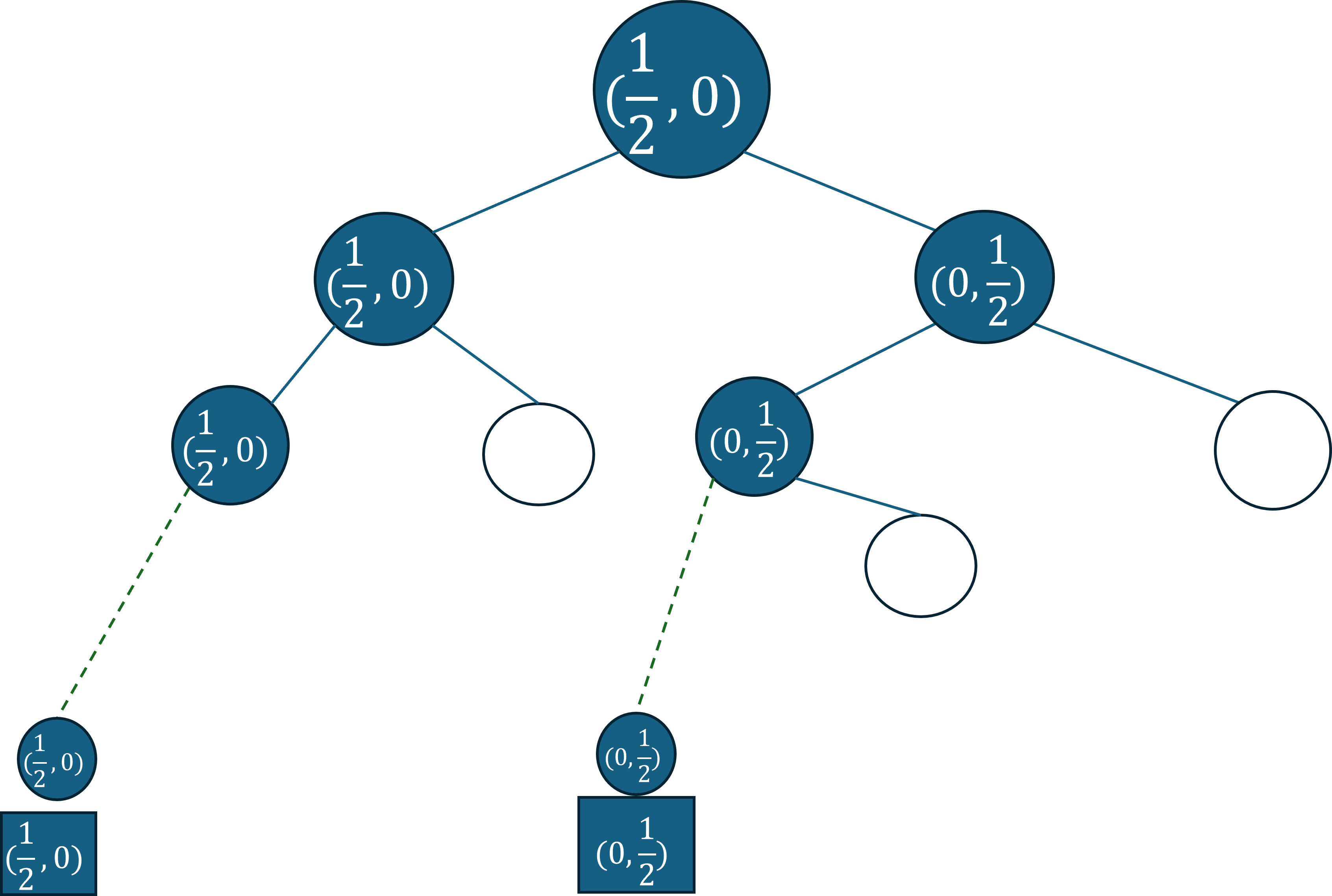
An example of an MBC tree is shown in Figure 1.
The Data Structure.
The overall data structure comprises a sequence of identical MBC trees , each of fixed height ,222All logarithms are with base unless otherwise mentioned. and with the roots labeled with balls of radius . The number of MBC trees is not fixed in advance; the sequence grows dynamically as needed.
Remark 3.
We assume , ensuring that the height of the MBC trees is non-negative.
2.1 The Online Metric TSP Algorithm
We assume knowledge of the value of the optimal solution in describing our algorithm in this section. In Appendix A, we will relax this assumption at the cost of an additional factor in the competitive ratio. We use to set the radius of the balls at the roots of the MBC trees in our data structure, i.e., in our data structure.
We now describe the online algorithm that inserts a point into the array using the sequence of MBC trees. The algorithm searches for a partial, admissible node of the lowest possible height across all existing MBC trees.
-
If such a node is found, we call , which is described below.
-
If no such node exists, we create a new MBC tree , add it to the sequence, and call .
Local Insertion ().
The procedure starts by identifying a node as follows:
-
If is a partial node, is the right child of .
-
Otherwise, is the root of a new tree; in this case, .
Starting from , the algorithm traverses down to a leaf by repeatedly choosing the left child. For every node on this path (including ), we mark with center and radius where is the height of . Finally, is stored at the leaf at the end of this path.
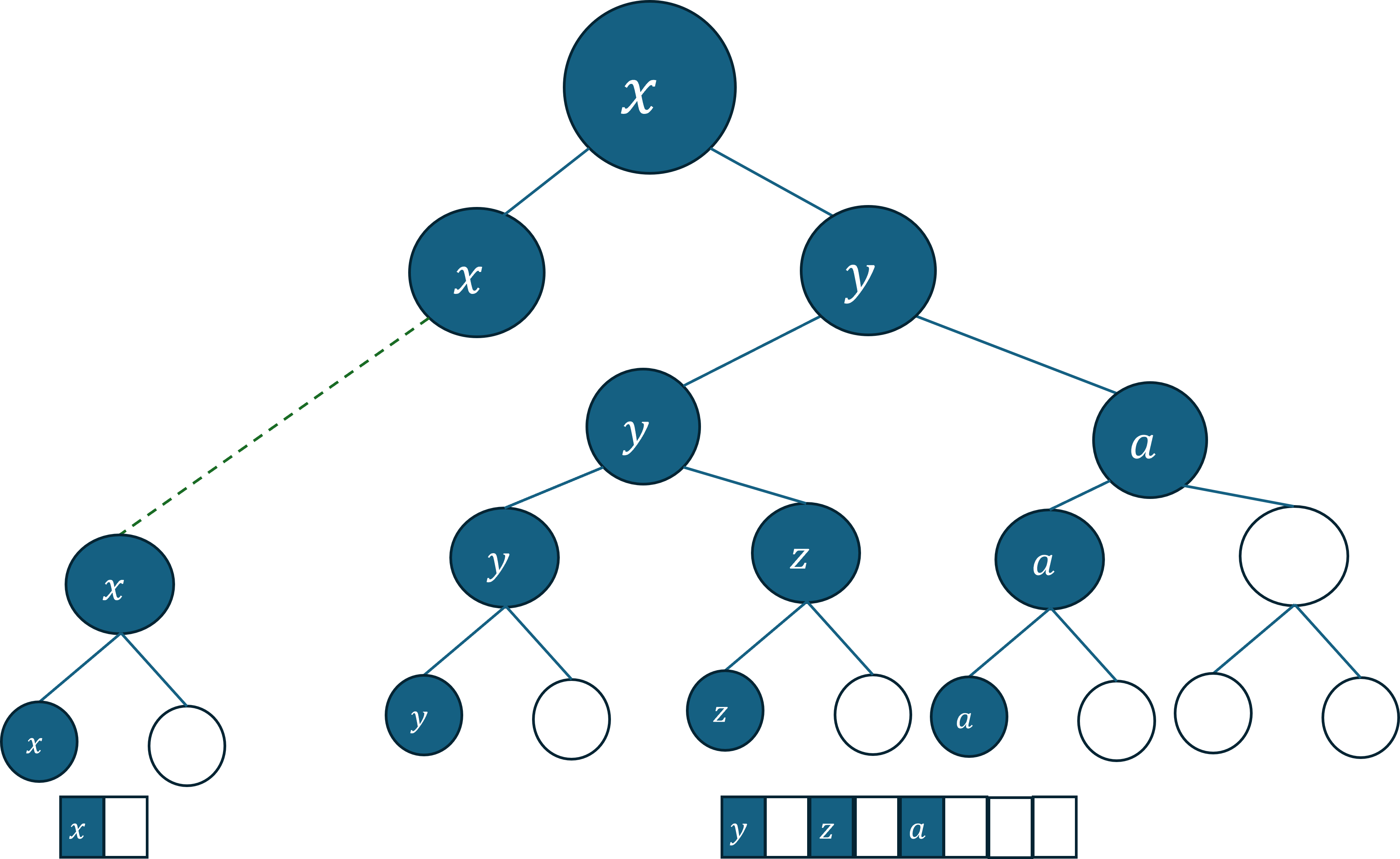
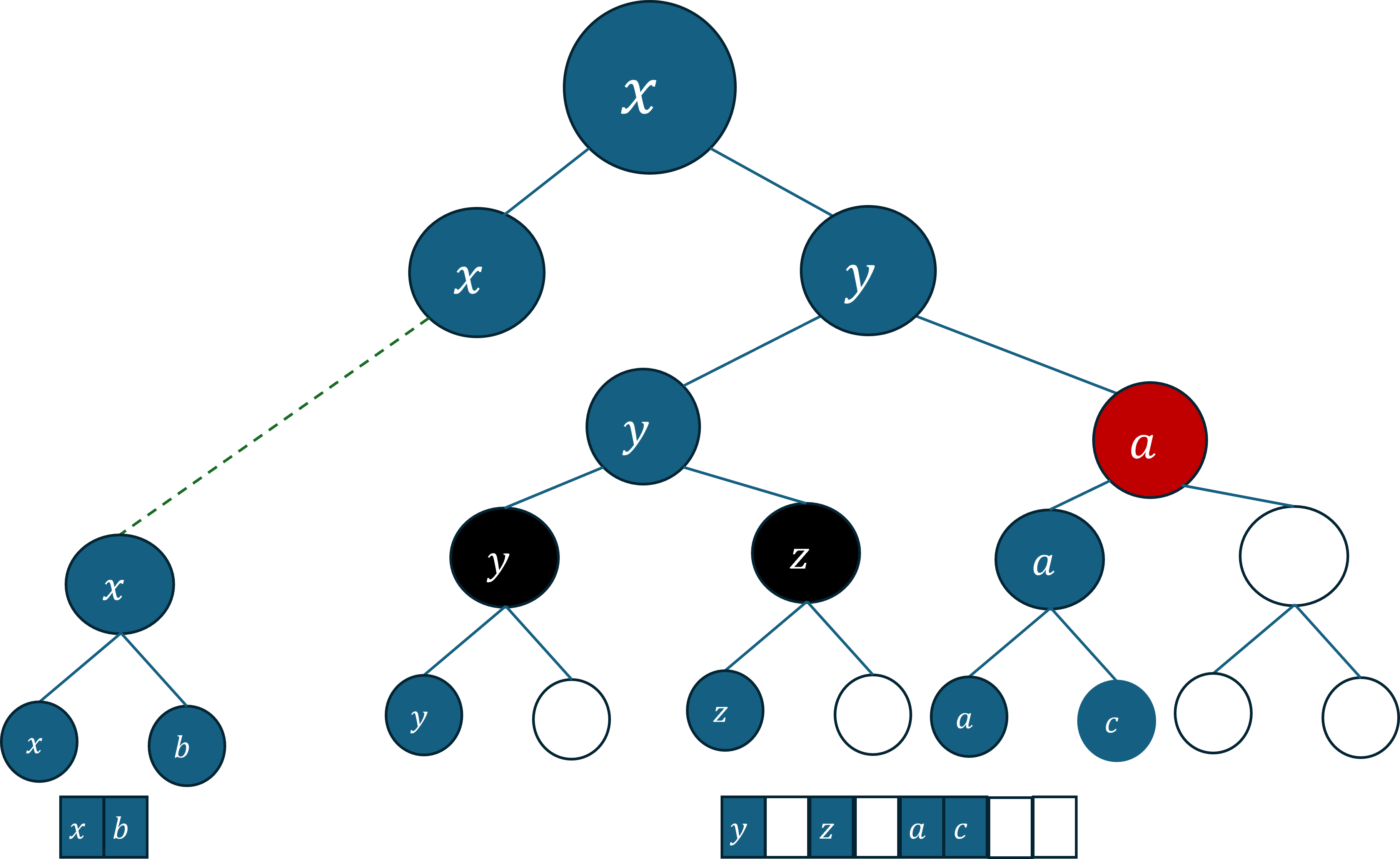
In Figure 2, we show the insertion of a new point in an MBC tree.
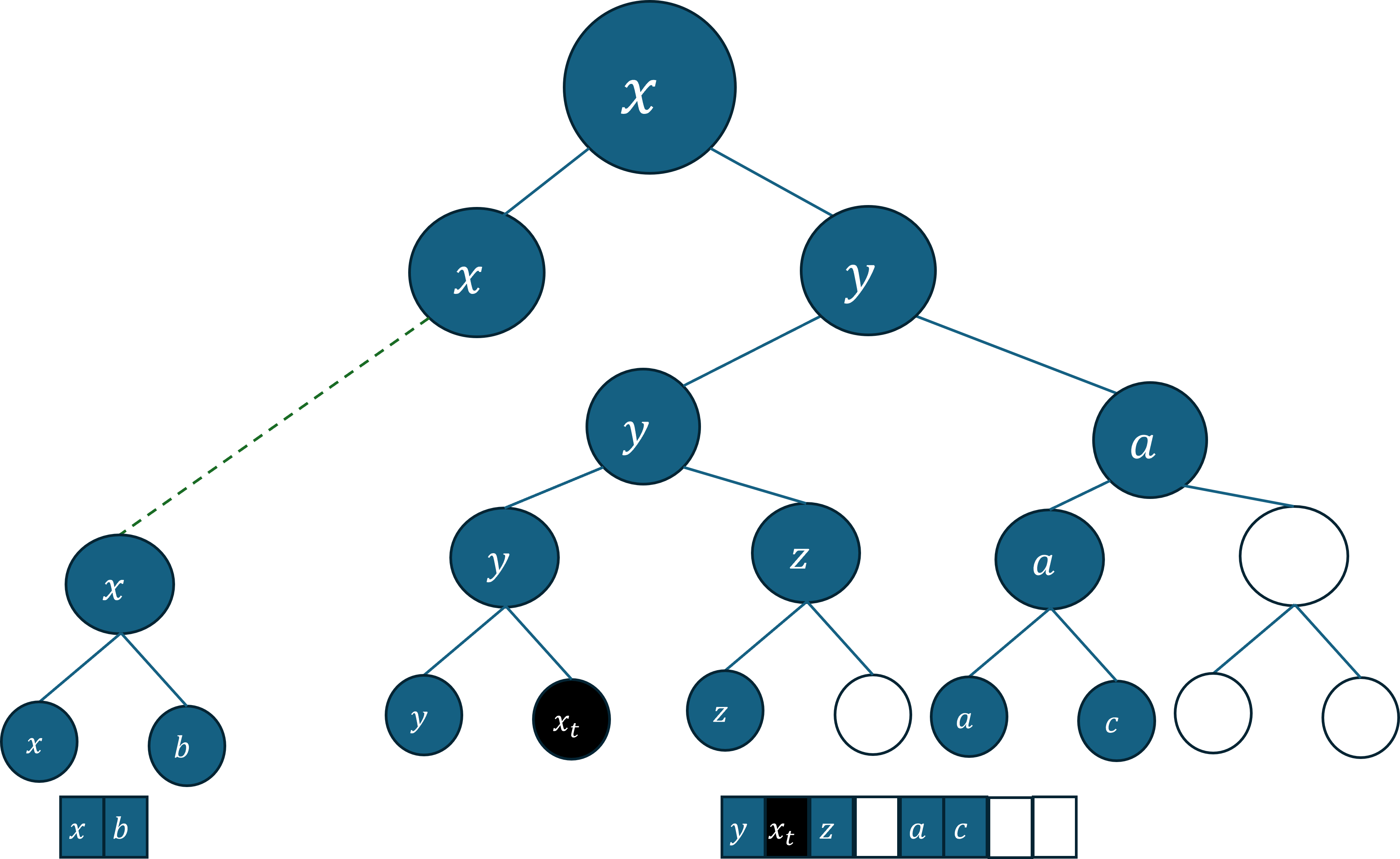
2.2 Space Usage of the Algorithm
We start by showing that the size of the array used by the online metric TSP algorithm is at most . For this, we bound the number of unused cells in the array. Note that each partial node has an unmarked child with an unused subarray under it. Conversely, the unused space in the array can be partitioned into subarrays that are subtended by the unmarked children of partial nodes. Therefore, it suffices to bound the cumulative unused space under unmarked children of partial nodes in the data structure.
Our main claim is the following:
Claim 4.
For all partial nodes at a fixed height , the cumulative unused space under their unmarked children is at most .
In order to prove this claim, we will use the following important property.
Claim 5.
Let and be two partial nodes (nodes with exactly one marked child) at the same height , with centers and . Then .
Proof.
Without loss of generality, assume was marked before (created by the insertion of a point ). When the algorithm attempted to insert , it checked all existing marked nodes at height , including . Since is partial, it had an available (unmarked) child, which means the insertion into would have succeeded if were admissible.
The fact that was not inserted in the subtree under , while the insertion algorithm prefers the partial node at the lowest possible height, implies that is inadmissible at . Therefore, . Since , it follows that .
Proof of Claim 4..
Let be the number of partial nodes at height . By Claim 5, their centers are points that are pairwise separated by distance . Since the optimal TSP tour (of cost ) visits all points, it must connect these centers incurring a cost . Substituting , we get .
Since each partial node at height has an unmarked child node at height that has unused array cells under it, the total unused space in the array is at most
We can now derive the space usage of the online algorithm from Claim 4.
Lemma 6.
The unused space in the array is at most at any time. As a consequence, the array uses at most space after inserting all points.
Proof.
By Claim 4, it follows that the total empty space is at most:
2.3 Competitive Ratio of the Algorithm
We want to prove the following bound:
Lemma 7.
The total cost of the solution produced by the algorithm is .
To prove this lemma, we first establish some important properties of the online algorithm.
Claim 8.
Let be two marked nodes in the MBC tree such that is the parent of . Then, the point at the center of the ball labeling must be admissible at .
Proof.
There are two possibilities. The first is that . In this case, the claim trivially holds. Otherwise, the labeling at was done by the procedure , which can only be run if is admissible at .
Claim 9.
Let be a point that is stored in the array cell at a leaf node of an MBC tree, and let be a node of height which is an ancestor of . Then .
Proof.
We will prove the claim by induction on . For the base case of , we have from Claim 8 that is admissible at . Therefore, .
Let denote the vertices on the path from a leaf to its ancestor at height . Let denote . By the inductive hypothesis, we have . Furthermore, using Claim 8, we know that . Therefore, by the triangle inequality,
Using the above claim, we establish a bound on the total cost within an MBC tree.
Lemma 10.
Suppose a set of points is inserted into an MBC tree of height . Then, the total cost of the points in is at most .
Proof.
Let be a pair of points that occupy consecutive non-empty cells in the array (the leaves of ). Let denote the least common ancestor of and in , and let be the left and right children of .
By the structure of the tree, is the rightmost non-empty leaf in the subtree rooted at , and is the leftmost non-empty leaf in the subtree rooted at . By Claim 9, we have and . Therefore, by the triangle inequality, we get
We charge this distance to the node . Every internal node in the MBC tree is charged at most once. Summing over all heights , we get that the total cost is at most
We now return to the proof of Lemma 7.
Proof of Lemma 7.
By Lemma 6, the total space used by the algorithm is at most . The size of the subarray under a single MBC tree of height is
Therefore, the number of MBC trees, denoted , is at most
We now sum the costs. The total cost consists of the cost within each MBC tree and the cost incurred between MBC trees.
1. Cost within MBC trees.
By Lemma 10, the cost of a single MBC tree is at most . Since , the cumulative internal cost across all trees is at most:
2. Cost between MBC trees.
We are left with the cost incurred between MBC trees, i.e., by the rightmost point in and the leftmost one in . For any pair of points, the distance is at most . Thus, the total cost between trees is at most
Adding these two types of cost, we get that the total cost is at most
3 Lower Bound for Online Sorting and Online Metric TSP
Recall from Section 1 that our lower bound that establishes Theorem 2 for online metric TSP is actually for the online sorting problem, i.e., on the line metric, Moreover, the lower bound explicitly assumes that the algorithm does not know the value of , and therefore, does not apply to prior results in online sorting that assume knowledge of .
Before proceeding further, we restate Theorem 2 for the online sorting problem, and also change notation in a way that will make it easier to describe the construction. The reader can easily verify that the theorem below implies Theorem 2.
Theorem 11.
Consider the online sorting problem on elements. Any deterministic online sorting algorithm that is competitive requires at least space, for any .
We will assume the terminology of an adversary and an arbitrary deterministic algorithm. In every step of the online instance, the adversary reveals a batch of new elements, which the algorithm inserts in empty cells of the array. This sequence repeats itself until the adversary decides to end the instance.
Epochs and Phases.
Overall, the online steps are organized in a sequence of epochs. Conceptually, the adversary achieves two properties in each epoch. First, it increases the range of elements from the previous epoch by a multiplicative factor. Second, because of the change in the overall range, all elements in the previous epochs become much smaller than all elements in the current range. In effect, this allows us to treat the elements in previous epochs as (being close enough to) , which helps simplify the analysis. More precisely, the elements presented by the adversary in the th epoch are in the range . Note that by induction, all elements in the previous epochs are in the range , which are at least far from every element in epoch .
An epoch is further subdivided into a sequence of phases. In each phase, the adversary presents a batch of elements, which are inserted by the algorithm in the array. We now describe the th phase of the th epoch. As stated previously, the range of elements in this epoch is . Let us call this range . For , the adversary presents elements, and . Subsequently, for every , the adversary presents a batch of elements that are all distinct such that the elements in all phases up to the th one are equally spaced in the range . In particular, the th element of the th epoch at the end of the th phase is given by where ranges from to . Note that any two consecutive elements in this epoch differ in their values by . In other words, the th phase supplies the missing elements such that the complete set accumulated by the end of the phase is given by , where ranges from to (We give a pictorial depiction of the elements arriving in different phases of an epoch in Figure 3.)

Real and Vacuous Holes.
This brings us to the crucial decision taken by the adversary after the algorithm inserts the elements presented in a phase. The adversary can perform three possible actions:
-
it can continue to the next phase of the current epoch,
-
it can terminate the current epoch and go to the first phase of the next epoch, or
-
it can terminate the instance altogether.
To describe the conditions for this decision, we need to define the notion of holes in the array:
A hole is a set of contiguous cells in the array all of which are vacant.
Initially, the whole array is a single hole. Over time, as the array fills up, this single hole gives rise to multiple holes. For notational convenience, we extend this terminology to say that two consecutive array cells that are both occupied also have a vacuous hole between them. In contrast, a hole that comprises an actual non-empty sequence of vacant array cells is called a real hole.
It will be useful to define categories of holes, both vacuous and real. First, we categorize holes into three types based on the elements at their two ends:
-
Mixed Holes. These are holes where one end of the hole is occupied by an element from a previous epoch and the other end is occupied by an element from the current epoch.
-
New Holes. These are holes where both ends of the hole are occupied by elements from the current epoch.
-
Old Holes. These are holes where both ends of the hole are occupied by elements from a previous epoch.
Second, orthogonally to the previous categorization, we group holes based on their size:
-
Large Holes. These are holes that contain at least (vacant) array cells. (By definition, all large holes are real holes.)
-
Small Holes. These are holes that contain fewer than (vacant) array cells.
We define the phase of a hole based on its endpoints: a hole is considered to be created in phase of the current epoch if at least one of the elements defining its ends belongs to phase .
After the algorithm inserts the elements in the th phase of the th epoch, the adversary makes its next move according to the current state of the array. In particular, it uses the following conditions, which are checked in order:
-
Condition 1: If the array contains at least mixed holes (including both real and vacuous holes), then the adversary terminates the instance.
-
Condition 2: If the value of reaches , then the adversary terminates the instance.
-
Condition 3: If the array contains at least large new holes, then the adversary terminates the current epoch and goes to the first phase of the st epoch.
-
If none of the above conditions hold, then the adversary continues with the st phase of the current epoch.
To establish the lower bound in Theorem 11, we show two facts: first, that the instance ends with at most elements, and second, that the competitive ratio is at least .
Upper Bound on Number of Elements.
To show that the instance ends with at most elements, we first lower bound the number of large holes:
Claim 12.
Let denote the total number of elements already inserted at the time that the adversary switches from epoch to . Then, the number of large holes is at least .
Proof.
We prove this claim by induction on .
Suppose the current epoch ended with phases. Let denote the number of elements inserted in the current epoch. Since the adversary created a new epoch , by Condition 3, the number of large new holes at the end of epoch is at least . Now, note that by the inductive hypothesis, the number of large holes at the end of epoch was at least . All these holes become old holes at the beginning of epoch . If an element is inserted in such an old hole in epoch , then that creates at least mixed hole in epoch . (In fact, mixed holes are created unless the old hole is at one end, in which case only mixed hole is created.) Since Condition 1 was never satisfied, we can conclude that at most of these old holes have had insertion of elements in epoch . In other words, at least of the large old holes at the beginning of epoch have been untouched during epoch , and therefore, they continue to be large holes at the end of epoch .
We now sum the number of large holes at the end of epoch . The count includes the large new holes created during epoch and the large old holes from the beginning of epoch that were untouched during epoch . Thus, the total number of large holes at the end of epoch is at least , since for . This completes the inductive proof.
Next, we show that any single epoch cannot contribute more than elements. This shows that if the instance has elements overall, then all but of them must be from completed epochs.
Claim 13.
The maximum number of elements inserted in an epoch is at most .
Proof.
Note that an epoch ends if it reaches the beginning of the st phase. Thus, the number of elements in an epoch is at most the number of inserted elements till the end of the th phase. Since the total number of elements till the th phase is , it follows that the total number of elements in an epoch is at most . Using the above claims, we now show that the instance cannot have more than elements.
Lemma 14.
The number of elements in the instance constructed by the adversary has at most elements.
Proof.
Assume for contradiction that elements were inserted. Then, by Claim 13, at least elements were inserted in completed epochs. Then, by Claim 12, there are at least large holes at the end of the last completed epoch. Since each large hole has vacant array cells, it follows that the size of the array is at least
for . This contradicts the fact that the array is of size in the statement of Theorem 11.
Lower Bound on the Competitive Ratio.
Finally, we show that the competitive ratio is at least . We start with the case when the instance is terminated by the first condition:
Lemma 15.
If the array contains at least mixed holes, then the competitive ratio is at least .
Proof.
Recall that denotes the range for the current epoch . The elements in all the previous epochs are in the range . As a consequence, the difference between any element in the current epoch and any element in a previous epoch is at least . Therefore, every mixed hole induces a cost of at least .
Now, note that optimal cost is at most the maximum value in the current range , i.e., . Since there are at least mixed holes, the total cost is at least , which implies a competitive ratio of at least .
Next, we consider the case where the instance is terminated by the second condition. Note that in this case, the third condition did not hold at the end of the th phase that immediately preceded the current phase. (Otherwise, the adversary would have moved to the next epoch.) We establish the following claim, which yields a lower bound of the cost of the algorithm based on the index of the current phase.
Claim 16.
Suppose . Then, if the array contains fewer than large new holes after inserting the elements in the th phase of epoch , then the cost of the algorithm is at least .
Proof.
In this proof, we obtain a lower bound on the cost by only considering small new holes, and disregarding all other types of holes. Specifically, in each phase, we account only for the cost of small holes newly created during that phase. Once a small new hole is created in a phase, further subdivisions of this hole in subsequent phases are not counted, since these might not cause additional cost.
Suppose we are at the end of the th phase. If epoch did not end after phase , then conditions 1 and 3 did not hold at the end of this phase. Therefore, there can be at most large new holes, in addition to at most mixed holes. Since elements were inserted in the current epoch, the number of small new holes is at least:
| (3.1) |
where the inequality holds for any , since for .
Observe that inserting an element into an empty cell within an existing small new hole does not incur any additional cost if the element’s value lies between those of the elements at its two ends. Consequently, to derive a valid lower bound for the cost in phase , we exclude from our analysis all elements inserted into small holes that were created during the first phases. However, if an element is inserted in an existing large new hole, and this creates a small new hole, this does increase the cost since we explicitly excluded the cost of all large holes from the analysis. Likewise, if the insertion of elements into a mixed hole creates a small new hole, we also include its cost in our accounting.
So, we want to discard small new holes of two types from the above count: (a) those that have elements from a previous phase before at either end, and (b) those that were created in the current phase by inserting elements in phase into a small new hole that existed at the end of phase . We count these together by counting the total number of cells that were one of two types at the end of phase : (a) either a vacant cell in a small new hole or (b) an occupied cell at one end of a small new hole.
The number of elements inserted in the current epoch up to phase is given by:
Therefore, the number of small new holes at the end of phase is at most , since each new hole has an element from the current epoch on each side. Note that each small new hole has at most vacant cells. Therefore, the total number of cells that are either vacant in a small new hole or at one end of a small new hole at the end of phase is at most:
| (3.2) |
Subtracting (3.2) from (3.1), we get that the number of small new holes that incur additional cost in the th phase is at least:
where the inequality holds since .
Next, we determine the minimum cost per hole. The elements in range are uniformly spaced such that the minimum difference between any two distinct elements in phase is
Multiplying the number of contributing holes by the minimum cost per hole, the total cost accumulated strictly within phase is at least
Multiplying by the number of phases, the total cost is at least .
Using the above claim, we immediately get the following:
Lemma 17.
If the algorithm terminates with , then the competitive ratio of the algorithm is at least .
Proof.
This is an immediate corollary of Claim 16. Specifically, if reaches , then the cost at the end of the last completed phase is at least .
4 Closing Remarks
In this paper, we explored the tradeoff between competitive ratio and space usage for the online metric TSP problem. In particular, we gave a deterministic algorithm that uses space and improves the competitive ratio from (for space) to . We also showed that this cannot be improved further to -competitiveness using a deterministic algorithm, unless the space used increases to for constant .
Our work raises several interesting questions. First, our lower bound only applies to deterministic algorithms; we believe that the lower bound might also hold for randomized algorithms, but the current construction does not readily extend to the randomized setting. Second, while we rule out -competitive deterministic algorithms with , it is quite possible that setting for some constant yields an -competitive algorithm. Indeed, improving on the competitive ratio of [24, 14], even with unlimited space usage, remains open.
References
- [1] Anders Aamand, Mikkel Abrahamsen, Lorenzo Beretta, and Linda Kleist. Online sorting and translational packing of convex polygons. In Nikhil Bansal and Viswanath Nagarajan, editors, Proceedings of the 2023 ACM-SIAM Symposium on Discrete Algorithms, SODA 2023, Florence, Italy, January 22-25, 2023, pages 1806–1833. SIAM, 2023. doi:10.1137/1.9781611977554.CH69.
- [2] Mikkel Abrahamsen, Ioana O. Bercea, Lorenzo Beretta, Jonas Klausen, and László Kozma. Online sorting and online TSP: randomized, stochastic, and high-dimensional. In Timothy M. Chan, Johannes Fischer, John Iacono, and Grzegorz Herman, editors, 32nd Annual European Symposium on Algorithms, ESA 2024, September 2-4, 2024, Royal Holloway, London, United Kingdom, volume 308 of LIPIcs, pages 5:1–5:15. Schloss Dagstuhl – Leibniz-Zentrum für Informatik, 2024. doi:10.4230/LIPIcs.ESA.2024.5.
- [3] Sanjeev Arora, Carsten Lund, Rajeev Motwani, Madhu Sudan, and Mario Szegedy. Proof verification and the hardness of approximation problems. J. ACM, 45(3):501–555, 1998. doi:10.1145/278298.278306.
- [4] Giorgio Ausiello, Esteban Feuerstein, Stefano Leonardi, Leen Stougie, and Maurizio Talamo. Algorithms for the on-line travelling salesman. Algorithmica, 29(4):560–581, 2001. doi:10.1007/S004530010071.
- [5] Yossi Azar. Lower bounds for insertion methods for TSP. Comb. Probab. Comput., 3:285–292, 1994. doi:10.1017/S096354830000119X.
- [6] Yossi Azar, Debmalya Panigrahi, and Or Vardi. Nearly tight bounds for the online sorting problem. In Proceedings of the 2026 Annual ACM-SIAM Symposium on Discrete Algorithms (SODA), pages 6642–6658. SIAM, 2026. doi:10.1137/1.9781611978971.237.
- [7] Christian Bertram. Online metric TSP. In Anne Benoit, Haim Kaplan, Sebastian Wild, and Grzegorz Herman, editors, 33rd Annual European Symposium on Algorithms, ESA 2025, Warsaw, Poland, September 15-17, 2025, LIPIcs, pages 80:1–80:9. Schloss Dagstuhl – Leibniz-Zentrum für Informatik, 2025. doi:10.4230/LIPIcs.ESA.2025.80.
- [8] Antje Bjelde, Jan Hackfeld, Yann Disser, Christoph Hansknecht, Maarten Lipmann, Julie Meißner, Miriam Schlöter, Kevin Schewior, and Leen Stougie. Tight bounds for online TSP on the line. ACM Trans. Algorithms, 17(1):3:1–3:58, 2021. doi:10.1145/3422362.
- [9] Michiel Blom, Sven Oliver Krumke, Willem de Paepe, and Leen Stougie. The online TSP against fair adversaries. INFORMS J. Comput., 13(2):138–148, 2001. doi:10.1287/IJOC.13.2.138.10517.
- [10] Nicos Christofides. Worst-case analysis of a new heuristic for the travelling salesman problem. Operations Research Forum, 3, 1976. URL: https://api.semanticscholar.org/CorpusID:123194397.
- [11] Esteban Feuerstein and Leen Stougie. On-line single-server dial-a-ride problems. Theor. Comput. Sci., 268(1):91–105, 2001. doi:10.1016/S0304-3975(00)00261-9.
- [12] Dimitris Fotakis, Andreas Kalavas, Charalampos Platanos, and Thanos Tolias. A polylogarithmic algorithm for stochastic online sorting, 2025. doi:10.48550/arXiv.2508.12527.
- [13] Yang Hu. Nearly optimal bounds for stochastic online sorting, 2025. arXiv:2508.07823.
- [14] Makoto Imase and Bernard M. Waxman. Dynamic steiner tree problem. SIAM J. Discret. Math., 4(3):369–384, 1991. doi:10.1137/0404033.
- [15] Patrick Jaillet and Michael R. Wagner. Generalized online routing: New competitive ratios, resource augmentation, and asymptotic analyses. Oper. Res., 56(3):745–757, 2008. doi:10.1287/OPRE.1070.0450.
- [16] Anna R. Karlin, Nathan Klein, and Shayan Oveis Gharan. A (slightly) improved approximation algorithm for metric TSP. Oper. Res., 72(6):2543–2594, 2024. doi:10.1287/OPRE.2022.2338.
- [17] Marek Karpinski, Michael Lampis, and Richard Schmied. New inapproximability bounds for TSP. J. Comput. Syst. Sci., 81(8):1665–1677, 2015. doi:10.1016/J.JCSS.2015.06.003.
- [18] Sven Oliver Krumke, Willem de Paepe, Diana Poensgen, and Leen Stougie. News from the online traveling repairman. Theor. Comput. Sci., 295:279–294, 2003. doi:10.1016/S0304-3975(02)00409-7.
- [19] Sven Oliver Krumke, Luigi Laura, Maarten Lipmann, Alberto Marchetti-Spaccamela, Willem de Paepe, Diana Poensgen, and Leen Stougie. Non-abusiveness helps: An o(1)-competitive algorithm for minimizing the maximum flow time in the online traveling salesman problem. In Klaus Jansen, Stefano Leonardi, and Vijay V. Vazirani, editors, Approximation Algorithms for Combinatorial Optimization, 5th International Workshop, APPROX 2002, Rome, Italy, September 17-21, 2002, Proceedings, volume 2462 of Lecture Notes in Computer Science, pages 200–214. Springer, 2002. doi:10.1007/3-540-45753-4_18.
- [20] Maarten Lipmann. On-line routing. PhD thesis, Technische Universiteit Eindhoven, Eindhoven, The Netherlands, 2003.
- [21] Nicole Megow, Martin Skutella, José Verschae, and Andreas Wiese. The power of recourse for online MST and TSP. SIAM J. Comput., 45(3):859–880, 2016. doi:10.1137/130917703.
- [22] Jubayer Nirjhor and Nicole Wein. Improved online sorting, 2025.
- [23] Christos H. Papadimitriou and Mihalis Yannakakis. The traveling salesman problem with distances one and two. Math. Oper. Res., 18(1):1–11, 1993. doi:10.1287/MOOR.18.1.1.
- [24] Daniel J. Rosenkrantz, Richard Edwin Stearns, and Philip M. Lewis II. An analysis of several heuristics for the traveling salesman problem. SIAM J. Comput., 6(3):563–581, 1977. doi:10.1137/0206041.
- [25] Anatolii Ivanovich Serdyukov. Some extremal bypasses in graphs. Upravlyaemye Sistemy, 17:76–79, 1978. [in Russian].
Appendix A The general case for unknown
In this section, we extend the result in Section 2 to the case of unknown , at the cost of an additional factor of in the competitive ratio.
Following [6], we apply a doubling scheme on the value of the optimal solution. The doubling scheme uses two parameters: the optimal cost and the number of inserted points for a given guess on . We have an outer loop that (at least) doubles the estimate on in each iteration, and an inner loop that doubles the number of inserted points. This nested doubling process is initialized after sequentially inserting the first two points (in the first two array cells); twice their distance provides an initial estimate for .
Each iteration of the outer loop is called an epoch. Since MBC trees are not defined for small values of (see Remark 3), we start any epoch by inserting the first points consecutively before starting the doubling scheme. In the -th epoch, the guess on is denoted . When the arrival of a new point causes the estimated cost (defined as twice the cost of the minimum spanning tree on the points seen so far) to exceed , the -th epoch ends and the -st epoch starts. The value of in the new epoch is set to be at least double that of the previous epoch. Each epoch is assigned new space in the array, which begins immediately after the last cell used in the previous epoch.
Within an epoch, each iteration of the inner loop is called a phase. Let denote the bound on the number of inserted points in the -th phase of the -th epoch. The phase ends when the number of points exceeds , and the -st phase starts with . Overall, we define .
In the -th phase, we allocate a new subarray that begins immediately after the subarray used in the -st phase. The amount of space allocated in the -th phase is . During the -th phase, we employ the algorithm from Section 2 for inserting points with the variable (instead of ) as a black box.
In the proofs below, we use to respectively denote the number of phases and points in the -th epoch, and to denote the number of points in its -th phase.
Lemma 18 (Space Bound).
The algorithm inserts points in space.
Proof.
By Lemma 6, in phases , the unused space is at most times the used space, and in phase , it is at most times . But, , i.e., the unused space in phase is at most times the used space in this epoch. Thus, the total unused space is at most an -fraction of the used space in this epoch. The lemma follows.
Lemma 19 (Cost Bound).
The cost incurred by the algorithm is at most .
Proof.
Fix epoch . The cost between consecutive phases is at most , based on the current bound on the optimal solution. This results in a total additive cost of at most between the phases. In addition, since we insert the first points sequentially, we incur an additional cost of at most . Finally, there is a cost of within each phase by Lemma 7. Therefore, the total cost in the -th epoch is at most
In addition, the cost between epochs and is at most . Summing over all epochs, we get that the total cost is at most
Note that at least doubles in every epoch, and at any time it provides a -approximation to the true value of . As a result, . Moreover, the total number of phases in any epoch is at most , i.e., for every . Applying these facts to the above cost bound, we get that the total cost is at most
Appendix B A Counter-Example to the Analysis from [6] for a General Metric Space
The upper bound analysis in [6] relies on the structural property that all partial nodes at any height are labeled by disjoint intervals. The adaptation of this key property into balls for a general metric is used in our paper as well in Claim 5. However, the insertion algorithm from [6], adapted to general metrics, does not maintain this key property.
First, we recall the insertion algorithm from [6]. The procedure is defined as follows:
-
If is a leaf node and is unmarked, then label with the left or right half of its parent’s label that contains , write in the array cell at the leaf node , and return success.
-
If is marked and is inadmissible at , then return failure.
-
If is marked and is admissible at , then call . If it returns success, return success. Otherwise, if it returns failure, then call . If this returns success, then return success. Otherwise, if it returns failure as well, then return failure.
-
If is unmarked, then label with the left or right half of its parent’s label that contains and call .
In short, attempts to insert first to the left child of and then to the right child of . Note that this operation also applies for balls as labels instead of intervals. As usual, the overall data structure comprises a series of identical MBC trees . Let be the point being inserted. The algorithm in [6] iterates over the subarrays corresponding to these trees in order, i.e., it attempts to insert in , then , then , etc., until the point is successfully inserted.
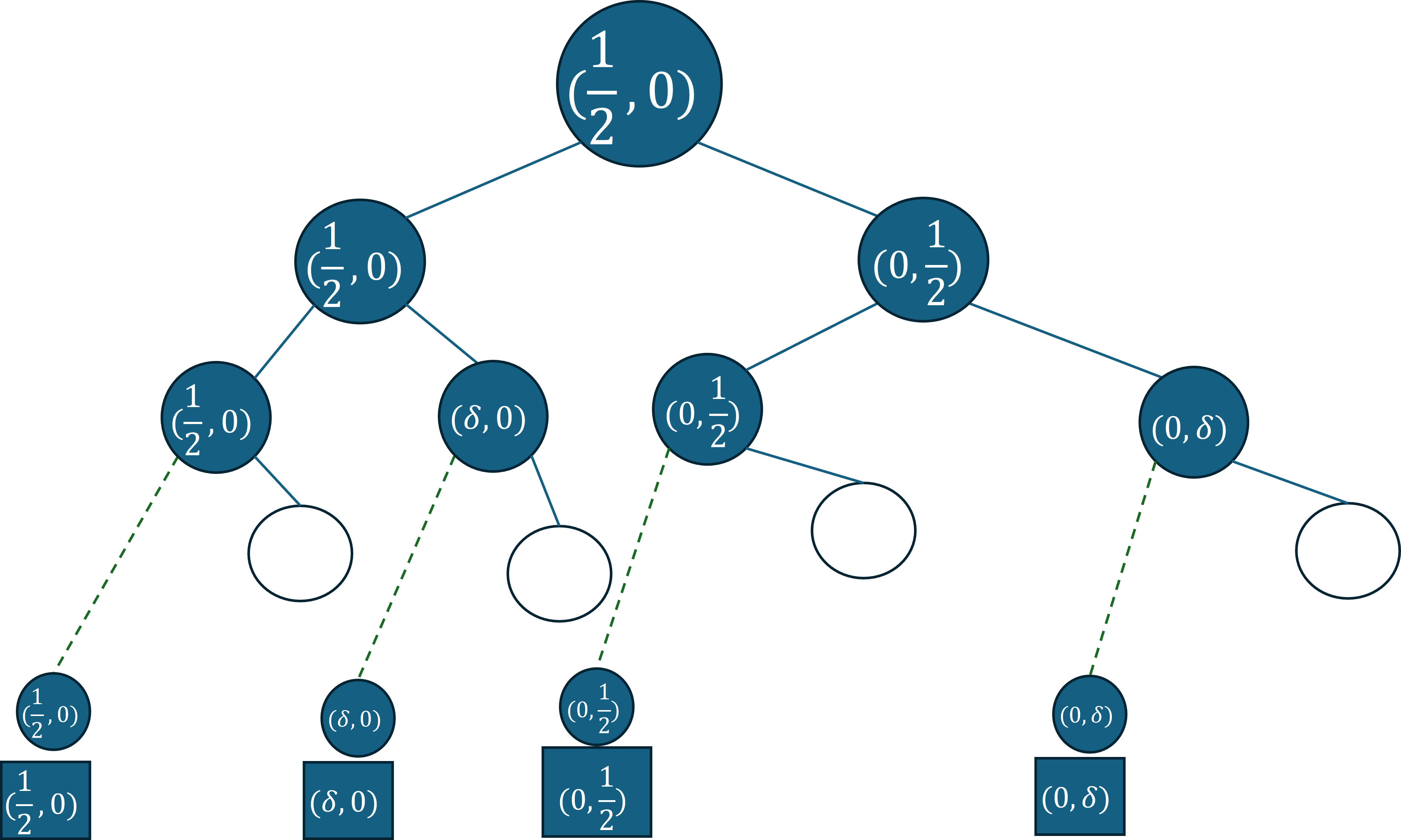
We now demonstrate that the distance property claimed in Claim 5 fails for this insertion algorithm for with the metric.
The instance starts by inserting . As shown in Figure 4, these two points mark two sibling nodes (call these ) in the MBC tree with balls of radius and centered at respectively. Next, we insert the points for a small . Observe that , whereas . Thus, is inserted under and creates a partial node (call it ) labeled by a ball centered at . Similarly, is inserted under and creates a partial node (call it ) labeled by a ball centered at . The two partial nodes at the same height contradict Claim 5 since the points are only at distance from each other.