On the Average-Case Performance of Greedy for Maximum Coverage

Balkanski, Eric; Chatzitheodorou, Jason; Sentenac, Flore

doi:10.4230/LIPIcs.ICALP.2026.20

On the Average-Case Performance of Greedy for Maximum Coverage

Eric Balkanski

Columbia IEOR, New York, NY, USA Jason Chatzitheodorou

Columbia IEOR, New York, NY, USA Flore Sentenac

HEC, Paris, France

Abstract

For the classical maximum coverage problem, the greedy algorithm achieves a worst-case $1-1/e$ approximation, which is optimal unless $\text{P}=\text{NP}$ . The notion of coverage appears in a wide range of optimization tasks, where empirical evaluations indicate approximation ratios close to $1$ for the greedy algorithm on real data. Random models have provided average-case justifications for the empirical performance of many well-known algorithms, but little is known about the average-case performance of greedy for maximum coverage.

We analyze the expected approximation ratio of the greedy algorithm in a random model, which we call the left-regular random model. We first show that, for all parameter settings of this model, the expected approximation ratio of the greedy algorithm improves by a constant over its worst-case $1-1/e$ guarantee. We then identify two simple conditions, either of which ensures that the expected approximation ratio is close to $1$ for sufficiently large graphs. Finally, we show that there is a regime where greedy does not achieve an expected approximation better than $0.94$ . To obtain these results, we develop analytical tools, including a novel application of the differential equation method and a connection to maximum matching in Erdős-Rényi graphs, which may be of independent interest for other random models.

Keywords and phrases:

Maximum Coverage, Greedy Algorithm, Average-Case Analysis, Differential Equation Method, Random Graphs

Category:

Track A: Algorithms, Complexity and Games

Copyright and License:

2012 ACM Subject Classification:

Theory of computation

\rightarrow

Approximation algorithms analysis

Related Version:

Full Version: https://arxiv.org/abs/2604.24884

Funding:

Eric Balkanski and Jason Chatzitheodorou were supported in part by NSF grants CCF-2210501 and IIS-2147361.

DOI:

10.4230/LIPIcs.ICALP.2026.20

Event:

53rd International Colloquium on Automata, Languages, and Programming (ICALP 2026)

Editors:

Sayan Bhattacharya, Danupon Nanongkai, Michael Benedikt, and Gabriele Puppis

Series and Publisher:

Leibniz International Proceedings in Informatics, Schloss Dagstuhl – Leibniz-Zentrum für Informatik

1 Introduction

Maximizing coverage is a fundamental problem in computer science and operations research, as the notion of coverage arises across a wide range of optimization tasks. Influence maximization in social networks [17], facility and sensor placement [18], information retrieval [1], content recommendation [25], and finding essential webpages [4] are examples of problems that have been formulated as maximum coverage problems. Maximum coverage is also closely related to set cover, one of Karp’s original 21 NP-complete problems [16].

Maximum coverage can be defined as follows. Given a bipartite graph with left nodes $L$ and right nodes $R$ , the goal is to find the $k$ nodes in $L$ that cover the largest number of nodes in $R$ , i.e., $\max_{S\subseteq L:|S|\leq k}|N(S)|$ . The greedy algorithm, which iteratively selects the node in $L$ that covers the largest number of nodes in $R$ not yet covered, achieves a $1-1/e$ worst-case approximation ratio guarantee [21], which is optimal unless $\text{P}=\text{NP}$ [10]. However, worst-case guarantees are often driven by pathological instances, leading to pessimistic bounds that can be uninformative in practice. There have been numerous approaches to bridging this gap between theory and practice for various problems through beyond–worst-case analyses of algorithms. A canonical example is the smoothed analysis of the simplex method [26].

For maximum coverage, the greedy algorithm empirically performs significantly better than its $1-1/e$ approximation ratio guarantee [4, 5]. There have been numerous attempts going beyond worst-case to explain this strong performance in practice for the broader problem of monotone submodular maximization under a cardinality constraint. These include the parameterized properties of curvature [8], stability [7], and sharpness [23]. More recently, [24] considered a budget-smoothed model where the cardinality constraint $k$ is stochastic.

However, except for a few notable exceptions discussed in Section 1.1, little is known about the average-case performance of greedy for maximum coverage on random graphs. In contrast, random models have provided average-case justifications for the performance of classical algorithms such as quicksort [14], first-fit decreasing for bin packing [12], local search for the traveling salesman problem [9], and the greedy algorithm for both max-value [19, 2] and min-cost matching [13]. Motivated by the strong empirical performance of greedy for maximum coverage, we explore the following question.

What is the average-case performance of the greedy algorithm for maximum coverage?

We study the approximation ratio of greedy under a model that we call the left-regular random model $\textsc{LRR}(n,d)$ . This model generates a bipartite graph with $n$ left nodes $L$ and $n$ right nodes $R$ , where each node $u\in L$ independently selects $d$ neighbors uniformly at random from $R$ . We also consider extensions in which $|L|\neq|R|$ and the nodes in $L$ have non-uniform degrees. Our motivation for the $d$ -regularity assumption for left nodes $L$ in the base model is that it is a challenging regime for greedy. In particular, there are simple bad instances for greedy in which the left nodes have equal degree (see Section A.1 for an example). Moreover, in empirical evaluations of extensions of this model, greedy’s approximation ratio was lowest when the nodes in $L$ had equal degree (see Section A.2 for an example).

Our results

Our first main result is an unconditional bound on the expected approximation ratio of greedy in the left-regular random model. We show that for all values of $n, d,$ and $k$ , there is a constant improvement for the approximation ratio of greedy in this random model compared to its worst-case approximation ratio of $1-1/e$ . For all results, we assume that greedy breaks ties according to an arbitrary but consistent ordering of the nodes in $L$ .

Theorem 1.

There exists a constant $c>0$ such that for all $n\in\mathbb{N},d\in[n],k\in[n]$ , the greedy algorithm achieves, in expectation, a $(1-1/e+c)$ -approximation under the left-regular random model.

The second main result provides two alternative sufficient conditions, either of which ensures a near-optimal approximation ratio for greedy for sufficiently large graphs.

Theorem 2.

For any $\epsilon\in(0,1)$ , $n=\Omega(\epsilon^{-8})$ , the greedy algorithm achieves, in expectation, a $1-\epsilon$ approximation under the left-regular random model if either $d=\Omega(\epsilon^{-8})$ or $k\in\left[0,\frac{\epsilon n}{2d}\right]\cup\left[\frac{2n}{\epsilon d},\,n\right]$ .

This result implies that, for any constant $\epsilon$ , the degree $d$ of nodes in $L$ being super-constant or the cardinality constraint $k$ lying outside of a constant factor neighborhood of $n/d$ are sufficient conditions for a $1-\epsilon$ approximation. We note that when $k=n/d$ , then the sum of the degrees of $k$ left nodes is equal to the number of right nodes. The only regime for which Theorem 2 does not give near-optimality is where $d$ is constant and $k=\Theta(n/d)$ . The third main result shows that for $d=2$ and some $k$ such that $k=\Theta(n/d)$ , the approximation ratio of greedy is not near-optimal as $n$ grows large: it is upper bounded by $0.94$ .

Theorem 3.

For $d=2$ , there exists a sequence $k(n)$ of cardinality constraints such that the expected approximation ratio of the greedy algorithm is at most $0.94$ in the limit as $n\rightarrow\infty$ under the left-regular random model.

These results indicate that the left-regular random model is sufficient to always get a constant improvement in the approximation ratio of greedy, but that it requires additional assumptions for near-optimality; Theorem 2 gives two such assumptions.

Extensions

In the full version of our paper, we consider two extensions of the left-regular random model.

$\blacksquare$

Unbalanced bipartite graphs. We consider an extension $\textsc{ULRR}(n,m,d)$ of the base model $\textsc{LRR}(n,d)$ where the number of right nodes is denoted by $m$ and is potentially different from the number of left nodes $n$ . We show that for all $n, m$ such that $n=cm$ for some constant $c>0$ and for all $d\in[m]$ and $k\in[n]$ , there exists a constant $\epsilon_{c}>0$ such that greedy achieves a $1-1/e+\epsilon_{c}$ approximation in expectation.
$\blacksquare$

Non-regular unbalanced bipartite graphs. We consider an extension $\textsc{GenR}(n,m,\{d_{i}\}_{i\in[n]})$ of the base model where the left nodes have degree $d_{1}\geq\cdots\geq d_{n}$ and the bipartite graph is unbalanced. We show that if either (1) the sum of the $k$ largest degrees is bounded away from $m$ : $\sum_{i=1}^{k}d_{i}\not\in[(\epsilon/2)m,(\epsilon/2)^{-1}m]$ , (2) the average degree of the $k$ largest degrees is sufficiently large: $\frac{1}{k}\sum_{i=1}^{k}d_{i}=\Omega(\max(1,(n/m)^{2})\epsilon^{-8})$ , or (3) $d_{1},\ldots,d_{n}$ are drawn from a power law distribution and $k$ is sufficiently small, then the expected approximation ratio of greedy is at least $1-\epsilon$ .

Our techniques

The positive results rely on two main analytical tools, which may also be of interest for analyzing greedy in other random bipartite graph models.

First, we develop a framework using the differential equation method to analyze an AcceptReject algorithm that is equivalent to greedy. AcceptReject proceeds in phases; in each phase, it iterates through every node to either add it to the solution or reject it. We show that the evolution of the value of the current solution of AcceptReject during the first phase can be approximated by a function that is the unique solution to a differential equation. This differential equation is obtained by approximating the expected per-iteration increase in the solution size as a function of the current solution size.

Second, we show that greedy’s expected value is at least the expected value of a fixed set of $k$ left nodes, chosen independently of the random graph’s realization. Although this claim may seem intuitive, it requires a careful argument because there are iterations in which the marginal gain of the fixed set is larger than that of greedy, where these marginal gains are measured with respect to their respective current solutions. We circumvent that obstacle by analyzing a hybrid algorithm that runs greedy for $t$ iterations and then completes the solution by selecting the $k-t$ nodes with the largest residual degrees at iteration $t$ .

The negative result is established by relating maximum coverage in $2$ -left regular graphs and maximum matching in Erdős-Rényi random graphs. This connection yields a lower bound on the coverage of the optimal solution via known results on maximum matching. At the same time, we tightly control the performance of greedy through our differential equation analysis.

Open questions

An alternative random model in which it would be natural to study the approximation ratio of greedy is the Erdős–Rényi random bipartite graph model $G_{n,n,p}$ with $n$ left nodes, $n$ right nodes, and an edge between each left and right node independently with probability $p$ . To the best of our knowledge, there is no known result for the maximum coverage problem under Erdős–Rényi random bipartite graphs and analyzing greedy in that model seems non-trivial.

Obtaining stronger unconditional bounds on the approximation ratio of greedy in the left-regular random model is a natural direction for future work. In particular, using the differential equation method to analyze additional phases of AcceptReject is a promising direction for establishing stronger approximation guarantees for greedy in the regime where it is not near-optimal.

Paper organization

We discuss additional related work in Section 1.1 and introduce preliminary definitions and notation in Section 2. In Section 3, we show the approximation guarantees achieved by greedy in the left-regular random model. In Section 4, we show the negative result for greedy.

1.1 Related Work

[4] use the dual of the maximum coverage LP to provide bounds on the approximation ratio of greedy that are in practice much stronger than its worst-case $1-1/e$ approximation. In particular, for $k\geq 50$ , they obtain bounds on real data that are always at least $0.95$ . They also show that in the random model, where left nodes and right nodes both have degrees that follow a power law distribution and edges are added randomly according to these degree distributions, greedy achieves a $1-\epsilon$ approximation if it has a marginal contribution of at least $O(\epsilon^{-2}\log n)$ at every iteration. In [27], three algorithms for maximum coverage, including greedy, are analyzed heuristically using the differential equation method on sparse biregular random bipartite graphs. In particular, they use a differential equation to predict a threshold for the cardinality constraint $k$ below which greedy achieves exact optimality with high probability and above which it is no longer optimal with high probability.

For the closely related set cover problem where the goal is to cover all the nodes in $R$ with a subset of $L$ of minimum size, [11] and [6] also study a random model with fixed degrees and also use the differential equation method. However, their primary focus is on methods that, given parameter values for the random model, yield numerical estimates of the approximation ratio of greedy on random instances for these specific parameters, but not closed-form approximation ratios. In addition to these numerical estimates, [11] shows that for a fixed ratio $|R|/|L|$ , greedy is asymptotically optimal as the degree of right nodes tends to infinity. When each edge is included with constant probability, [28] shows that there is an algorithm, distinct from greedy, that is asymptotically optimal for set cover.

2 Preliminaries

In the maximum coverage problem, there is a bipartite graph $B=(L,R,E)$ with $n$ left nodes $L=\{u_{1},\ldots,u_{n}\}$ , $m$ right nodes $R=\{v_{1},\ldots,v_{m}\}$ , and edges $E\subseteq L\times R$ . The goal is to find the $k$ nodes in $L$ that cover the largest number of nodes in $R$ , i.e., $\max_{S\subseteq L:|S|\leq k}|N_{B}(S)|$ where $N_{B}(S)$ are the neighbors of $S$ in $B$ . We abuse notation and write $N(S)$ when $B$ is clear from context. The greedy algorithm (Greedy) iteratively adds to the current solution $S$ the left node that covers the most right nodes not yet covered. We refer to $|N(u)\setminus N(S)|$ and $|N(S)|$ as the marginal contribution of $u$ to $S$ and the value of $S$ , respectively.

Algorithm 1

\text{{Greedy}}(B,k)

.

The random graph model

We consider instances of the maximum coverage problem with random bipartite graphs drawn from the following random graph model that we call the left-regular random model. Throughout the paper, uppercase letters represent fixed sets/graphs, while calligraphic letters denote random sets/graphs.

Definition 4.

The $\textsc{LRR}(n,d)$ model generates a bipartite graph $\mathcal{B}=(L,R,\mathcal{E})$ by setting $|L|=|R|=n$ and, independently for each $u\in L$ , selecting $d$ neighbors in $R$ uniformly at random without replacement.

We note that a left-regular random graph satisfies $\Pr\left[v_{j}\in N(u_{i})\right]=\frac{d}{n}$ for all $v_{j}\in R$ and $u_{i}\in L$ . When analyzing Greedy under the left-regular random model, we assume it breaks ties according to an arbitrary, but consistent, ordering of the nodes in $L$ , and that the left nodes $u_{i}$ are indexed in the order in which greedy breaks ties.

We let $\mathcal{G}_{k}(\mathcal{B})$ and $\mathcal{O}_{k}(\mathcal{B})$ denote the greedy solution and the optimal solution, respectively, for the maximum coverage problem with cardinality constraint $k$ over a bipartite graph $\mathcal{B}\sim\textsc{LRR}(n,d)$ . Throughout the paper, approximation guarantees in expectation are defined as ratios of expected values. For fixed $n, d,$ and $k$ , the greedy algorithm achieves, in expectation, an $\alpha$ -approximation if

\operatorname{\mathbb{E}}\limits_{\mathcal{B}\sim\textsc{LRR}(n,d)}[|N(% \mathcal{G}_{k}(\mathcal{B}))|]\geq\alpha\cdot\operatorname{\mathbb{E}}\limits% _{\mathcal{B}\sim\textsc{LRR}(n,d)}[|N(\mathcal{O}_{k}(\mathcal{B}))|].

We abuse notation and write $\mathcal{G}_{k}$ and $\mathcal{O}_{k}$ when $\mathcal{B}$ is clear from context. It will be useful in our analysis to compare $\operatorname{\mathbb{E}}[|N(\mathcal{G}_{k})|]$ to the expected value of a fixed set of size $k$ . For that purpose, we denote the first $k$ left nodes as $H_{k}=\{u_{1},u_{2},\dots,u_{k}\}.$ We also use the notation $[n]=\{1,\ldots,n\}$ .

3 Approximation Guarantees

In this section, we show that greedy achieves an approximation ratio that is, for all parameters $n, d$ , and $k$ , a constant improvement over its worst-case $1-1/e$ guarantee and, in a wide range of regimes, asymptotically optimal. We first discuss two central technical tools that we use for these two results in Section 3.1, then partition the space of all parameters in three regions and analyze greedy in each of them in Section 3.2, and finally combine the analyses of these regions to obtain the desired results in Section 3.3. Missing proofs can be found in the full version of our paper.

3.1 Technical Tools

The near-linear, saturated, and critical regions

We distinguish three parameter regimes that we analyze separately. First, for small values of $k$ , we have the near-linear region, where Greedy selects nodes that have neighborhoods with almost no overlap. Therefore, their value increases almost linearly with $k$ . Second, for large values of $k$ , we have the saturated region, where Greedy covers almost all the right nodes. Between these two regions lies the critical region, which is the most challenging to analyze.

The differential equation method

The first technical tool is a novel application of the differential equation method. We use it to estimate the number of iterations

t_{d}=\max\{t\geq 1:|N(\mathcal{G}_{t}(\mathcal{B}))\setminus N(\mathcal{G}_{t% -1}(\mathcal{B}))|=d\}

in which Greedy, over a left-regular random graph $\mathcal{B}\sim\text{{LRR}}(n,d)$ , selects a node with marginal contribution to the current solution $\mathcal{G}_{t-1}$ that is equal to $d$ , i.e., all $d$ neighbors of the selected node are disjoint from the neighbors of $\mathcal{G}_{t-1}$ . The main lemma for this estimate $t^{*}_{d}$ of $t_{d}$ is a bound on its error $|t_{d}-t^{*}_{d}|$ that, for any $d\leq\sqrt{n/2}$ , has an $\tilde{O}(\sqrt{n})$ dependence on $n$ with high probability.

Lemma 5.

Let $n\in\mathbbm{N}$ , $d\leq\sqrt{n/2},k\in[n]$ and $\mathcal{B}\sim\text{{LRR}}(n,d)$ . With probability at least $1-\frac{1}{n}$ , estimate $t^{*}_{d}=\left(1-\left(1+d(d-1)\right)^{-\frac{1}{d-1}}\right)\cdot\frac{n}{d}$ is such that $|t_{d}-t^{*}_{d}|\leq 3e^{d^{2}}\cdot\sqrt{8n\log{2n}}$ .

This estimate plays a key role in the proof showing that greedy achieves a constant improvement over $1-1/e$ in the critical region when $d$ is small. To prove Lemma 5, we employ the differential equation method, formalized by [29]. Under appropriate regularity conditions, including bounded increments and Lipschitz continuity, this method yields a high-probability bound on the discrepancy between a discrete stochastic process and the deterministic solution of an associated differential equation. It has found great use in the field of random graphs [11, 22, 29, 30, 19, 3].

We do not apply the method directly to the standard description of Greedy because its evolution is difficult to express through a low-dimensional Markovian state, which is crucial for tractability. Instead, we analyze AcceptReject, an equivalent reformulation of Greedy. AcceptReject, which is formally defined in Algorithm 2, proceeds in phases from $p=\max_{u\in L}|N(u)|$ to $1$ . In phase $p$ , it iterates over the left nodes $u_{i}$ of the bipartite graph in the order in which greedy breaks ties and either accepts (meaning a node gets added to the solution) or rejects each of them based on whether their marginal contribution to the current solution $A$ is at least $p$ . This iterative exploration of the graph in each phase implies that its randomness is revealed sequentially, allowing low-dimensional Markovian states to describe the evolution of the current solution size $|A|$ .

Algorithm 2

\text{{AcceptReject}}(B,k)

.

We denote by $\mathcal{A}^{p}_{i}$ the set $A$ of accepted nodes at iteration $i$ of phase $p$ of AcceptReject. For the proof of Lemma 5, we focus on analyzing the first phase $p=\max_{u\in L}|N(u)|=d$ of AcceptReject on a graph $\mathcal{B}\sim\text{{LRR}}(n,d)$ .

Proof sketch of Lemma 5 (proof can be found in the full version).

The solution returned by Greedy and AcceptReject is not only the same, but the ordering in which nodes are added to this solution is also identical since the nodes $u_{i}$ are indexed in the order in which Greedy breaks ties. Thus, the number of iterations $t_{d}$ where Greedy adds nodes with marginal contribution $d$ is equal to the number of nodes accepted during the first phase $p=d$ of AcceptReject, i.e., $t_{d}=|\mathcal{A}^{d}_{n}|$ . We define the function $F(y)=\left(1-dy\right)^{d}$ for all $y\in\mathbbm{R}$ .

The central part of the proof consists of showing that $|\mathcal{A}^{d}_{i}|\approx n\cdot y(i/n)$ where $y(\cdot)$ is the unique solution to the following differential equation:

\displaystyle y^{\prime}(t)=F(y(t))=\left(1-d\cdot y(t)\right)^{d},\ y(0)=0.

This approximation is obtained by using the differential equation method, which requires the following four conditions.

$\blacksquare$

The expected one-step change $\operatorname{\mathbb{E}}\!\left[|\mathcal{A}^{d}_{i+1}|\!-\!|\mathcal{A}^{d}_% {i}|\middle||\mathcal{A}^{d}_{i}|\right]$ is tightly approximated by $F\left(|\mathcal{A}^{d}_{i}|/n\right)$ . For this condition, we show the following:

$\displaystyle\operatorname{\mathbb{E}}\left[|\mathcal{A}^{d}_{i+1}|\!-\!|% \mathcal{A}^{d}_{i}|\middle||\mathcal{A}^{d}_{i}|\right]$ $\displaystyle=\Pr\left[|N(u_{i+1})\!\setminus\!N(\mathcal{A}^{d}_{i})|=d% \middle||\mathcal{A}^{d}_{i}|\right]$

$\displaystyle=\frac{\binom{n-|\mathcal{A}^{d}_{i}|d}{d}}{\binom{n}{d}}$

$\displaystyle\approx\left(1\!-\!\frac{d|\mathcal{A}^{d}_{i}|}{n}\right)^{d}$

$\displaystyle=F\left(\frac{|\mathcal{A}^{d}_{i}|}{n}\right).$
$\blacksquare$

The function $F$ is Lipschitz.
$\blacksquare$

A deterministic bound for the one-step change $|\mathcal{A}^{d}_{i+1}|-|\mathcal{A}^{d}_{i}|$ . In our case, $|\mathcal{A}^{d}_{i+1}|-|\mathcal{A}^{d}_{i}|\leq 1$ .
$\blacksquare$

$|\mathcal{A}^{d}_{0}|\approx y(0)$ . In our case, $|\mathcal{A}^{d}_{0}|=y(0)=0$ .

We show that $\mathcal{A}^{d}_{i}$ and $F$ satisfy these four conditions with parameters such that the resulting approximation $t_{d}=|\mathcal{A}^{d}_{n}|\approx n\cdot y(1)$ is sufficiently tight to imply the desired bound. $\hfill\blacktriangleleft$ A promising direction for future work is to leverage estimates of the number of accepts across all phases, rather than only the first, as this could yield a tighter lower bound on the coverage of Greedy. The main challenge is that the solution of the differential equations in each phase depends on the solutions from the preceding phases, making closed-form expressions analogous to those obtained for $t_{d}$ unlikely. This interdependence substantially complicates the derivation of the approximation ratio. Nevertheless, we believe that a sufficiently careful analysis could overcome these technical obstacles and uncover the true extent of the improvement that Greedy achieves over $1-1/e$ .

The fixed-set lower bound

The second technical tool provides a seemingly simple lower bound on the expected value of the greedy solution. The lower bound is the expected value of a fixed set of left nodes chosen independently of the realization of the random graph. For this fixed set of nodes, we consider the $k$ nodes with lowest indices $H_{k}=\{u_{1},\dots,u_{k}\}$ .

Lemma 6.

Let $n\in\mathbbm{N}$ , $d\in[n],k\in[n]$ , and $\mathcal{B}\sim\text{{LRR}}(n,d)$ , then $\operatorname{\mathbb{E}}\left[|N(\mathcal{G}_{k})|\right]\geq\operatorname{% \mathbb{E}}\left[|N(H_{k})|\right]$ .

In Section 3.2, we use this bound to show that greedy is near-optimal in the near-linear, the saturated, and the critical region when $d$ is large. The only region where it does not provide a constant improvement is in the critical region when $d$ is small, where we use Lemma 5 instead.

It may seem natural that Greedy performs better than $H_{k}$ over left-regular random graphs. However, a difficulty that arises in proving Lemma 6, is that the expected marginal improvement $\operatorname{\mathbb{E}}[|N(\mathcal{G}_{t})\setminus N(\mathcal{G}_{t-1})|]$ of Greedy is not always larger than the expected marginal improvement $\operatorname{\mathbb{E}}[|N(H_{t})\setminus N(H_{t-1})|]$ of $H_{k}$ at all iterations $t$ , which we illustrate in the full version of our paper. Nevertheless, in the early iterations, where a small number of right nodes have been covered, it does hold that $\operatorname{\mathbb{E}}[|N(\mathcal{G}_{t})\setminus N(\mathcal{G}_{t-1})|]% \geq\operatorname{\mathbb{E}}[|N(H_{t})\setminus N(H_{t-1})|]$ . The challenge is thus to show that the expected value of Greedy remains larger in later iterations.

Proof sketch of Lemma 6 (proof can be found in the full version).

We define a hybrid algorithm $\mathcal{Y}^{t}$ that runs in two phases. First, it runs $t$ iterations of Greedy, after which its current solution is $\mathcal{G}_{t}$ . In the second phase, it adds to the solution the $k-t$ nodes with largest marginal contribution to $\mathcal{G}_{t}$ .

The main part of the proof consists in showing that trading one iteration of Greedy in the first phase for one more node in the second phase reduces the expected value, i.e.,

\operatorname{\mathbb{E}}\left[|N(\mathcal{Y}^{t})|\right]\geq\operatorname{% \mathbb{E}}\left[|N(\mathcal{Y}^{t-1})|\right].

To show that inequality, we first note that $\mathcal{G}_{t}\subseteq\mathcal{Y}^{t}\cap\mathcal{Y}^{t-1}$ , which implies that it suffices to compare the marginal contribution of the $k-t$ other nodes in the two solutions to $\mathcal{G}_{t}$ . The crucial difference that we leverage is that the $k-t$ other nodes in $\mathcal{Y}^{t}$ are selected to be the nodes with largest marginal contribution to $\mathcal{G}_{t}$ , whereas for $\mathcal{Y}^{t-1}$ they are the nodes with largest marginal contribution to $\mathcal{G}_{t-1}$ . With $\operatorname{\mathbb{E}}\left[|N(\mathcal{Y}^{t})|\right]\geq\operatorname{% \mathbb{E}}\left[|N(\mathcal{Y}^{t-1})|\right],$ the lemma then follows since $\operatorname{\mathbb{E}}\left[|N(\mathcal{G}_{k})|\right]=\operatorname{% \mathbb{E}}\left[|N(\mathcal{Y}^{k})|\right]$ and $\operatorname{\mathbb{E}}\left[|N(\mathcal{Y}^{0})|\right]=\operatorname{% \mathbb{E}}\left[|N(H_{k})|\right].$ $\hfill\blacktriangleleft$

3.2 Analysis For The Different Regions

Near-linear and saturated regions

In both regions, we show that Greedy achieves a ratio close to $1$ in Lemma 7. Intuitively, in the near-linear region (i.e., $k<<n/d$ ), even the nodes of $H_{k}$ share very few neighbors; therefore, the expected value of Greedy is close to $k d$ . On the other hand, in the saturated region (i.e., $k>>n/d$ ), $H_{k}$ covers most of the right nodes, even if the nodes of $H_{k}$ share many neighbors.

Lemma 7.

Let $\epsilon\in(0,1),n\in\mathbbm{N},d\in[n],k\in\left[0,\frac{\epsilon n}{2d}% \right]\cup[\frac{2n}{\epsilon d},n]$ and $\mathcal{B}\sim\text{{LRR}}(n,d)$ . Then we have $\operatorname{\mathbb{E}}\left[|N(\mathcal{G}_{k})|\right]\geq\left(1-\epsilon% \right)\cdot\operatorname{\mathbb{E}}\left[|N(\mathcal{O}_{k})|\right]$ .

The proof uses the fixed set lower bound from Lemma 6, whose value is lower bounded by the following lemma (proof can be found in the full version).

Lemma 8.

Let $n\in\mathbbm{N}$ , $d\in[n],k\in[n]$ , and $\mathcal{B}\sim\text{{LRR}}(n,d)$ . Then $\operatorname{\mathbb{E}}\left[|N(H_{k})|\right]\geq\left(1-e^{-\frac{kd}{n}}% \right)\cdot n$ .

The proof also uses the following inequality, whose proof can be found in the full version.

Claim 9.

For all $\epsilon\in(0,1)$ , $\frac{1-e^{-\epsilon}}{\epsilon}\geq 1-\epsilon$ .

We are now ready to prove Lemma 7.

Proof of Lemma 7.

For $k\geq\frac{2n}{\epsilon d}$ :

\displaystyle\operatorname{\mathbb{E}}\left[|N(\mathcal{G}_{k})|\right]\geq% \operatorname{\mathbb{E}}\left[|N(H_{k})|\right]\geq\left(1-e^{-kd/n}\right)n% \geq\left(1-e^{-1/\epsilon}\right)\cdot n\geq\left(1-\epsilon\right)\cdot% \operatorname{\mathbb{E}}\left[|N(\mathcal{O}_{k})|\right],

where the first inequality is because $\operatorname{\mathbb{E}}\left[|N(\mathcal{G}_{k})|\right]$ is lower bounded by $\operatorname{\mathbb{E}}\left[|N(H_{k})|\right]$ by Lemma 6, the second inequality is due to Lemma 8, the third inequality is because $kd/n\geq 2/\epsilon\geq 1/\epsilon$ by assumption, the fourth inequality is due to $e^{-1/\epsilon}\leq\epsilon$ and $|N(\mathcal{O}_{k})|$ is upper bounded by $n$ . For $k\leq\frac{\epsilon n}{2d}$ :

	$\displaystyle\operatorname{\mathbb{E}}\left[\|N(\mathcal{G}_{k})\|\right]\geq% \operatorname{\mathbb{E}}\left[\|N(H_{k})\|\right]\geq\left(1-e^{-kd/n}\right)n=% \frac{1-e^{-kd/n}}{kd/n}\cdot kd$	$\displaystyle\geq\frac{1-e^{-\epsilon}}{\epsilon}\cdot kd$
		$\displaystyle\geq\left(1-\epsilon\right)\cdot\operatorname{\mathbb{E}}\left[\|N% (\mathcal{O}_{k})\|\right],$

where the first inequality is because $\operatorname{\mathbb{E}}\left[|N(\mathcal{G}_{k})|\right]$ is lower bounded by $\operatorname{\mathbb{E}}\left[|N(H_{k})|\right]$ by Lemma 6, the second inequality is due to Lemma 8, the third inequality is because $kd/n\leq\epsilon/2\leq\epsilon$ by assumption, the fourth inequality is due to Claim 9 and $|N(\mathcal{O}_{k})|$ is upper bounded by $k d$ . $\hfill\blacktriangleleft$

Critical region: large degrees

We use Lemma 6 and Chernoff bounds over negatively correlated variables to show a $1-\epsilon$ ratio in the critical region (i.e. $k\approx n/d$ ) when the degrees are large. Intuitively, it is possible to upper bound the optimal solution, since any $k$ nodes suffer from sharing too many neighbors.

Lemma 10.

Let $\epsilon\in(0,1),d\geq\frac{20^{4}}{\epsilon^{8}},n\geq d,k\in\left[\frac{% \epsilon n}{2d},\frac{2n}{\epsilon d}\right],$ and $\mathcal{B}\sim\text{{LRR}}(n,d)$ . Then we have $\operatorname{\mathbb{E}}\left[|N(\mathcal{G}_{k})|\right]\geq\left(1-\epsilon% \right)\cdot\operatorname{\mathbb{E}}\left[|N(\mathcal{O}_{k})|\right]$ .

Proof sketch (proof can be found in the full version).

We show that the values of all sets concentrate with high probability. To this end, we express the value $|N(S)|=\sum_{v\in R}\mathbbm{1}\{v\in N(S)\}$ of a set $S$ as the sum over $v\in R$ of the indicator variables for whether $v$ is covered by $S$ . We first show that these indicator variables are negatively correlated.

We then use a generalization of the Chernoff bound for negatively correlated variables and a union bound to show that $\Pr\left[|N(\mathcal{O}_{k})|\geq(1+\delta)\cdot\operatorname{\mathbb{E}}\left% [|N(H_{k})|\right]\right]\leq\frac{1}{n}$ for an appropriate choice of $\delta$ . It then follows that $\operatorname{\mathbb{E}}\left[|N(\mathcal{G}_{k})|\right]\geq\operatorname{% \mathbb{E}}\left[|N(H_{k})|\right]\geq\frac{1}{1+\epsilon}\operatorname{% \mathbb{E}}\left[|N(\mathcal{O}_{k})\right]$ , where the first inequality is by Lemma 6 and the second inequality by the choice of $\delta$ and the assumption on $n$ . $\hfill\blacktriangleleft$

Critical region: small degrees

We use Lemma 5 to lower bound the ratio in the critical region, when the degrees are small. The main challenge in this case is that the optimal solution can achieve a high value close to $n$ , so Lemmas 6 and 8 only retrieve worst-case ratio $1-\frac{1}{e}$ . Therefore, we need a tighter lower bound for Greedy. This is the most challenging case and the only one in which we do not show a $1-\epsilon$ ratio. Nevertheless, we still improve over the $1-\frac{1}{e}$ ratio by a constant, albeit small.

Lemma 11.

There exists a function $n_{0}(x):(0,1)\rightarrow\mathbbm{N}$ such that for $\epsilon\in(0,1),n\geq n_{0}(\epsilon),d\leq\frac{20^{4}}{\epsilon^{8}},k\in% \left[\frac{\epsilon n}{2d},\frac{2n}{\epsilon d}\right],$ and $\mathcal{B}\sim\text{{LRR}}(n,d)$ , we have $\operatorname{\mathbb{E}}\left[|N(\mathcal{G}_{k})|\right]\geq\left(1-\frac{1}% {e}+\Omega\left(\epsilon^{24}\right)\right)\cdot\operatorname{\mathbb{E}}\left% [|N(\mathcal{O}_{k})|\right]$ .

The proof uses worst-case analysis after iteration $t_{d}$ , to obtain a result for $k\geq t_{d}$ . Specifically, we show that as long as $t_{d}$ is on the order of $n/d$ , Greedy is bounded a constant away from $1-\frac{1}{e}$ , which we formalize in the following lemma.

Lemma 12.

Let $B=(L,R,E)$ be a $d$ -left-regular bipartite graph with $|L|=|R|=n$ . For all $k\geq t_{d}$ we have $|N(G_{k})|\geq\left(1-\frac{1}{e}+\frac{1}{e}\cdot\left(\frac{t_{d}}{n/d}% \right)^{3}\right)\cdot|N(O_{k})|$ .

We are now ready to give a proof sketch of Lemma 11.

Proof sketch of Lemma 11 (proof can be found in the full version).

Let $\delta$ be an appropriately chosen error term. For $k\leq t^{*}_{d}-\delta$ , Greedy gains $d$ on each iteration with high probability by Lemma 5, so $\operatorname{\mathbb{E}}\left[|N(\mathcal{G}_{k})|\right]\geq\left(1-\frac{1}% {n}\right)\cdot\operatorname{\mathbb{E}}\left[|N(\mathcal{O}_{k})|\right].$ For $k\geq t^{*}_{d}-\delta$ , Greedy gains $d$ on each iteration until $t^{*}_{d}-\delta$ with high probability by Lemma 5, and for later iterations we use Lemma 12:

\displaystyle\operatorname{\mathbb{E}}\left[|N(\mathcal{G}_{k})|\right]\geq% \left(1-\frac{1}{e}+\frac{1}{e}\cdot\left(\frac{t^{*}_{d}-\delta}{n/d}\right)^% {3}-\frac{8}{\epsilon n}\right)\cdot\operatorname{\mathbb{E}}\left[|N(\mathcal% {O}_{k})|\right].

We choose $n_{0}(\epsilon)$ large enough to make terms $\frac{\delta}{n/d}=O(\epsilon^{8})$ and $\frac{8}{\epsilon n}=O(\epsilon^{25})$ . The statement follows by lower bounding $\frac{t^{*}_{d}-\delta}{n/d}=\Omega(\epsilon^{8})$ . $\hfill\blacktriangleleft$

3.3 Putting Everything Together

By combining Lemma 7 and Lemma 10, we immediately get the near-optimality of greedy in the near-linear region, saturated region, and critical region with large degrees. See 2

The second main result regarding the approximation guarantee of greedy requires the following inequality (proof can be found in full version).

Claim 13.

For all $k\geq 1$ , $\left(1-\frac{1}{k}\right)^{k}\leq\frac{1}{e}-\frac{1}{4ek}$ .

By combining Lemma 11, which is for the critical region with small degrees, and Theorem 2, which is for all other regions, we get the constant improvement over $1-1/e$ for all regions.

Theorem 1. [Restated, see original statement.]

There exists a constant $c>0$ such that for all $n\in\mathbb{N},d\in[n],k\in[n]$ , the greedy algorithm achieves, in expectation, a $(1-1/e+c)$ -approximation under the left-regular random model.

Proof.

Let $\epsilon=0.3$ and $n_{0}(x)$ be the function from the statement of Lemma 11. For $n\geq n_{0}(\epsilon)$ , the statement is implied by Theorems 2 and 11. For $n<n_{0}(\epsilon)$ , the worst-case approximation ratio of greedy is $1-\left(1-\frac{1}{k}\right)^{k}$ , so we get

\displaystyle 1-\left(1-\frac{1}{k}\right)^{k}\geq 1-\frac{1}{e}+\frac{1}{4ek}% \geq 1-\frac{1}{e}+\frac{1}{4en_{0}(\epsilon)},

where the first inequality is by Claim 13 and the second since $k\leq n<n_{0}(\epsilon)$ . $\hfill\blacktriangleleft$

4 Limitation of Greedy

In the previous section, Theorem 2 does not guarantee an approximation ratio close to $1$ for all parameter values. The remaining difficult regime is when the degree $d$ is small and $k$ lies in a critical window around $n/d$ . In this section, we establish Theorem 3, which demonstrates that this gap is due to a fundamental limitation of Greedy rather than a proof artifact. Specifically, we identify a counterexample with $d=2$ , where the ratio is bounded away from $1$ as $n$ goes to infinity. The main results are Lemmas 15 and 17, which lower bound Opt and upper bound Greedy respectively. We defer the complete proofs to Appendix B.

4.1 Lower Bound for Opt

The first challenge is to lower-bound the value of the optimal solution. We resolve this difficulty by relating the value of the optimal solution in $2$ -left-regular random graphs to the size of a maximum matching in Erdős-Renyi random graphs. This process takes two steps.

First, the value of the optimal solution in any $2$ -left-regular bipartite graph $B=(L,R,E)$ is at least twice the minimum between $k$ and the size of the largest set of left nodes with no common neighbors, i.e.

\displaystyle|N(\mathcal{O}_{k}(B))|\geq 2\min\left(k,\lambda(B)\right),

(1)

with

\displaystyle\lambda(B)=\max\{|S|:S\subseteq L\text{ s.t. }N(u)\cap N(u^{% \prime})=\emptyset\ \forall u\neq u^{\prime}\in S\}.

(2)

The following lemma reduces the computation of $\lambda(B)$ to finding the size of a maximum matching in a specific graph $I_{B}$ , defined as follows: the vertex set of $I_{B}$ is the set of right nodes of $B$ , and for each left node $u\in L$ , we add an edge in $I_{B}$ between the two neighbors of $u$ . If two nodes on the left side share the same neighbor set, the parallel edges are merged; in other words, $I_{B}$ is a simple graph.

Lemma 14.

Let $B=(L,R,E)$ be a $2$ -left-regular bipartite graph. Also let $I_{B}=(R,E_{B})$ be a graph such that $E_{B}=\{e_{1},\dots,e_{n}\}$ where $e_{i}=N(u_{i})$ for all $i\in[n]$ . Then $\lambda(B)=\mu(I_{B})$ , where $\mu(I_{B})$ is the size of the maximum matching in $I_{B}$ .

Proof.

Consider a set $S\subseteq L$ attaining the maximum in Equation (2), i.e., $|S|=\lambda(B)$ and $N(u)\cap N(u^{\prime})=\emptyset$ for all distinct $u,u^{\prime}\in S$ . We construct

M=\{e_{i}:u_{i}\in S\},

which is a valid matching in $I_{B}$ by definition of $S$ , and clearly $|M|=|S|$ . We now show that $M$ is a maximum matching in $I_{B}$ . Towards a contradiction, assume there exists a matching $M^{\prime}$ in $I_{B}$ such that $|M^{\prime}|>|M|$ . Then we can define:

\displaystyle S^{\prime}=\{u_{i}:e_{i}\in M^{\prime}\},

where $N(u_{i})\cap N(u_{j})=\emptyset$ for all $u_{i},u_{j}\in S^{\prime}$ since $M^{\prime}$ is a matching. Then $|S^{\prime}|=|M^{\prime}|>|M|=|S|=\lambda(B)$ , which contradicts optimality of $S$ . The statement follows as $\lambda(B)=|S|=|M|=\mu(I_{B})$ . $\hfill\blacktriangleleft$

Now suppose that $\mathcal{B}$ is sampled from $\text{{LRR}}(n,2)$ . Then $\mathcal{I}_{\mathcal{B}}$ is distributed as a graph on $n$ vertices obtained by sampling $n$ edges independently and uniformly at random with replacement from the $\binom{n}{2}$ possible edges, merging parallel edges. This distribution is closely related to the classical Erdős–Rényi model $\mathbbm{G}_{n,m}$ , in which $m$ edges are sampled uniformly at random without replacement. Sharp estimates for the maximum matching size in Erdős–Rényi graphs are known; see, e.g., [15]. As we show in the following lemma, these results yield a bound on $\mu(\mathcal{I}_{\mathcal{B}})$ , which can be translated into a lower bound on the expected value of the optimal solution. Before we proceed, we define constants $\gamma_{*},\gamma^{*}$ , where $\gamma_{*}$ is the smallest root of $x=2e^{-2e^{-x}}$ and $\gamma^{*}=2e^{-\gamma_{*}}$ since we use them extensively in our proofs.

Lemma 15.

Let $n\in\mathbbm{N}$ and $\mathcal{B}\sim\text{{LRR}}\left(n,2\right)$ . Then for any $k\leq\left(1-\frac{\gamma^{*}+\gamma_{*}+\gamma^{*}\gamma_{*}}{4}-n^{-\frac{1}% {9}}\right)\cdot n$ , we have $\operatorname{\mathbb{E}}\left[|N(\mathcal{O}_{k})|\right]\geq(1-o(1))\cdot 2k.$

The proof leverages the following lemma, which provides a probabilistic lower bound on the size of the maximum matching in $\mathcal{I}_{\mathcal{B}}$ .

Lemma 16.

Let $n\in\mathbbm{N}$ and $\mathcal{B}\sim\text{{LRR}}\left(n,2\right)$ , then

\Pr\left[\mu(\mathcal{I}_{\mathcal{B}})\geq\left(1-\frac{\gamma^{*}+\gamma_{*}% +\gamma^{*}\gamma_{*}}{4}-n^{-\frac{1}{9}}\right)\cdot n\right]\geq 1-o(1).

The proof, deferred to Appendix B, bounds how much the maximum matching size can change due to the discrepancy between the generation process of $\mathcal{I}_{\mathcal{B}}$ and the seminal Erdős-Renyi model, and leverages what is known about the size of maximum matchings in Erdős-Renyi. We are now ready to prove Lemma 15.

Proof of Lemma 15.

Consider any $k\leq\left(1-\frac{\gamma^{*}+\gamma_{*}+\gamma^{*}\gamma_{*}}{4}-n^{-\frac{1}% {9}}\right)\cdot n$ , then:

\displaystyle\operatorname{\mathbb{E}}\left[|N(\mathcal{O}_{k})|\right]\geq 2k% \cdot\Pr\left[\lambda(\mathcal{B})\geq k\right]=2k\cdot\Pr\left[\mu(\mathcal{I% }_{\mathcal{B}})\geq k\right],

where the inequality is due to Equation 1 and the equality is due to $\lambda(\mathcal{B})=\mu(\mathcal{I}_{\mathcal{B}})$ by Lemma 14. We now lower bound $\mu(\mathcal{I}_{\mathcal{B}})$ :

\displaystyle\Pr\left[\mu(\mathcal{I}_{\mathcal{B}})\geq k\right]\geq\Pr\left[% \mu(\mathcal{I}_{\mathcal{B}})\geq\left(1-\frac{\gamma^{*}+\gamma_{*}+\gamma^{% *}\gamma_{*}}{4}-n^{-\frac{1}{9}}\right)\cdot n\right]\geq 1-o(1),

where the first inequality is due to the assumption on $k$ and the second due to Lemma 16. Chaining with the previous inequality establishes the lemma. $\hfill\blacktriangleleft$

4.2 Upper Bound for Greedy

The second challenge is to upper bound the value of Greedy. We do so through the machinery of Lemma 5 in the following lemma.

Lemma 17.

Let $n\in\mathbbm{N}$ and $\mathcal{B}\sim\text{{LRR}}\left(n,2\right)$ . Then we have that, for any $k>\frac{1}{3}\cdot n$ , $\operatorname{\mathbb{E}}\left[|N(\mathcal{G}_{k})|\right]\leq(1+o(1))\cdot% \left(\frac{1}{3}\cdot n+k\right)$ .

Proof.

By definition of $t_{2}$ , up to iteration $t_{2}$ , Greedy will gain $2$ per iteration, and thereafter it gains at most $1$ per iteration. Consequently, for any $k$ , the following holds

\mathbb{E}\left[|N(\mathcal{G}_{k})|\right]\leq\mathbb{E}\left[2t_{2}+(k-t_{2}% )\right]=\mathbb{E}[t_{2}]+k.

As $t_{2}\leq n$ always holds, we have:

\mathbb{E}[t_{2}]\leq t^{*}_{2}+3e^{4}\cdot\sqrt{8n\log{2n}}+n\cdot\Pr\left[t_% {2}\geq t^{*}_{2}+3e^{4}\cdot\sqrt{8n\log{2n}}\right].

We upper bound the probability using Lemma 5:

\Pr\left[t_{2}\geq t^{*}_{2}+3e^{4}\cdot\sqrt{8n\log{2n}}\right]\leq\frac{1}{n}.

Chaining those three inequalities yields:

\mathbb{E}\left[|N(\mathcal{G}_{k})|\right]\leq t^{*}_{2}+3e^{4}\cdot\sqrt{8n% \log{2n}}+1+k=\left(1+\frac{3e^{4}\cdot\sqrt{8n\log{2n}}+1}{t^{*}_{2}+k}\right% )(t^{*}_{2}+k).

The statement then follows, since $t^{*}_{2}=n/3$ by definition. $\hfill\blacktriangleleft$

4.3 Putting Everything Together

We proceed to show Theorem 3 by combining Lemmas 15 and 17. See 3

Proof.

Let $k(n)=\left\lfloor\left(1-\frac{\gamma^{*}+\gamma_{*}+\gamma^{*}\gamma_{*}}{4}-% n^{-\frac{1}{9}}\right)\cdot n\right\rfloor$ , then we have:

\displaystyle k(n)\geq\left(1\!-\!\frac{\gamma^{*}+\gamma_{*}+\gamma^{*}\gamma% _{*}}{4}\!-\!n^{-\frac{1}{9}}\right)\cdot n-1=\left(1\!-\!\frac{\gamma^{*}+% \gamma_{*}+\gamma^{*}\gamma_{*}}{4}\!-\!n^{-\frac{1}{9}}-n^{-1}\right)\cdot n.

(1)

We upper bound the ratio:

	$\displaystyle\frac{\operatorname{\mathbb{E}}\left[\|N(\mathcal{G}_{k(n)})\|% \right]}{\operatorname{\mathbb{E}}\left[\|N(\mathcal{O}_{k(n)})\|\right]}$	$\displaystyle\leq\frac{\operatorname{\mathbb{E}}\left[\|N(\mathcal{G}_{k(n)})\|% \right]}{(1-o(1))\cdot 2k(n)}$
		$\displaystyle\leq\frac{(1+o(1))\cdot\left(\frac{1}{3}\cdot n+k(n)\right)}{(1-o% (1))\cdot 2k(n)}$
		$\displaystyle\overset{n\rightarrow\infty}{\rightarrow}\frac{1}{2}+\frac{\frac{% 1}{3}}{2-\frac{\gamma^{}+\gamma_{}+\gamma^{}\gamma_{}}{2}}$
		$\displaystyle\leq 0.94,$

where the first inequality is due to Lemma 15, the second inequality is due to Lemma 17 which applies since $k(n)\geq t^{*}_{2}=\frac{1}{3}\cdot n$ for large enough $n$ , the limit is due to Equation (1) and because all $o(1)$ terms vanish, and the third inequality is because both $\gamma_{*},\gamma^{*}\leq 0.853$ . $\hfill\blacktriangleleft$

References

[1] Aris Anagnostopoulos, Luca Becchetti, Ilaria Bordino, Stefano Leonardi, Ida Mele, and Piotr Sankowski. Stochastic query covering for fast approximate document retrieval. ACM Trans. Inf. Syst., 33(3), 2015. doi:10.1145/2699671.
[2] Nick Arnosti. Greedy matching in bipartite random graphs. Stochastic Systems, 12(2):133–150, 2022.
[3] Jonathan Aronson, Alan Frieze, and Boris G Pittel. Maximum matchings in sparse random graphs: Karp–sipser revisited. Random Structures & Algorithms, 12(2):111–177, 1998. doi:10.1002/(SICI)1098-2418(199803)12:2\%3C111::AID-RSA1\%3E3.0.CO;2-\%23.
[4] Ricardo Baeza-Yates, Paolo Boldi, and Flavio Chierichetti. Essential web pages are easy to find. In Proceedings of the 24th International Conference on World Wide Web, WWW ’15, pages 97–107, 2015. doi:10.1145/2736277.2741100.
[5] Eric Balkanski, Sharon Qian, and Yaron Singer. Instance specific approximations for submodular maximization. In Marina Meila and Tong Zhang, editors, Proceedings of the 38th International Conference on Machine Learning, volume 139 of Proceedings of Machine Learning Research, pages 609–618. PMLR, July 2021. URL: http://proceedings.mlr.press/v139/balkanski21a.html.
[6] Joël Blot, Wenceslas Fernande de la Vega, Vangelis Th Paschos, and Rachid Saad. Average case analysis of greedy algorithms for optimisation problems on set systems. Theoretical computer science, 147(1-2):267–298, 1995. doi:10.1016/0304-3975(95)00242-O.
[7] Vaggos Chatziafratis, Tim Roughgarden, and Jan Vondrak. Stability and Recovery for Independence Systems. In 25th Annual European Symposium on Algorithms (ESA 2017), volume 87 of Leibniz International Proceedings in Informatics (LIPIcs), pages 26:1–26:15. Schloss Dagstuhl – Leibniz-Zentrum für Informatik, 2017. doi:10.4230/LIPIcs.ESA.2017.26.
[8] Michele Conforti and Gérard Cornuéjols. Submodular set functions, matroids and the greedy algorithm: tight worst-case bounds and some generalizations of the rado-edmonds theorem. Discrete applied mathematics, 7(3):251–274, 1984. doi:10.1016/0166-218X(84)90003-9.
[9] Matthias Englert, Heiko Röglin, and Berthold Vöcking. Worst case and probabilistic analysis of the 2-opt algorithm for the tsp. Algorithmica, 68(1):190–264, 2014. doi:10.1007/S00453-013-9801-4.
[10] Uriel Feige. A threshold of ln n for approximating set cover. J. ACM, 45(4):634–652, July 1998. doi:10.1145/285055.285059.
[11] W. Fernandez de la Vega, V. Th. Paschos, and R. Saad. Average case analysis of a greedy algorithm for the minimum hitting set problem. In Imre Simon, editor, LATIN ’92, pages 130–138, Berlin, Heidelberg, 1992. Springer Berlin Heidelberg.
[12] Greg N Frederickson. Probabilistic analysis for simple one-and two-dimensional bin packing algorithms. Information Processing Letters, 11(4-5):156–161, 1980. doi:10.1016/0020-0190(80)90041-1.
[13] Alan Frieze, Colin McDiarmid, and Bruce Reed. Greedy matching on the line. SIAM Journal on Computing, 19(4):666–672, 1990. doi:10.1137/0219045.
[14] Charles AR Hoare. Quicksort. The computer journal, 5(1):10–16, 1962. doi:10.1093/COMJNL/5.1.10.
[15] R. M. Karp and M. Sipser. Maximum matching in sparse random graphs. In 22nd Annual Symposium on Foundations of Computer Science (sfcs 1981), pages 364–375, 1981.
[16] Richard M Karp. Reducibility among combinatorial problems. Complexity of Computer Computations, pages 85–103, 1972. doi:10.1007/978-1-4684-2001-2_9.
[17] David Kempe, Jon Kleinberg, and Éva Tardos. Maximizing the spread of influence through a social network. In Proceedings of the Ninth ACM SIGKDD International Conference on Knowledge Discovery and Data Mining, 2003.
[18] Andreas Krause and Carlos Guestrin. Near-optimal observation selection using submodular functions. In Proceedings of the 22nd National Conference on Artificial Intelligence - Volume 2, 2007.
[19] Andrew Mastin and Patrick Jaillet. Greedy online bipartite matching on random graphs. arXiv preprint arXiv:1307.2536, 2013. arXiv:1307.2536.
[20] G. L. Nemhauser and L. A. Wolsey. Best algorithms for approximating the maximum of a submodular set function. Mathematics of Operations Research, 3(3):177–188, 1978. doi:10.1287/MOOR.3.3.177.
[21] G. L. Nemhauser, L. A. Wolsey, and M. L. Fisher. An analysis of approximations for maximizing submodular set functions – I. Mathematical Programming, 14:265–294, December 1978. doi:10.1007/BF01588971.
[22] Boris Pittel, Joel Spencer, and Nicholas Wormald. Sudden emergence of a giantk-core in a random graph. Journal of Combinatorial Theory, Series B, 67(1):111–151, 1996. doi:10.1006/JCTB.1996.0036.
[23] Sebastian Pokutta, Mohit Singh, and Alfredo Torrico. On the unreasonable effectiveness of the greedy algorithm: Greedy adapts to sharpness. In International Conference on Machine Learning, pages 7772–7782. PMLR, 2020. URL: http://proceedings.mlr.press/v119/pokutta20a.html.
[24] Aviad Rubinstein and Junyao Zhao. Budget-Smoothed Analysis for Submodular Maximization. In 13th Innovations in Theoretical Computer Science Conference (ITCS 2022), volume 215 of Leibniz International Proceedings in Informatics (LIPIcs), pages 113:1–113:23. Schloss Dagstuhl – Leibniz-Zentrum für Informatik, 2022. doi:10.4230/LIPIcs.ITCS.2022.113.
[25] Barna Saha and Lise Getoor. On maximum coverage in the streaming model & application to multi-topic blog-watch. In Proceedings of the SIAM International Conference on Data Mining, SDM 2009, April 30 - May 2, 2009, Sparks, Nevada, USA, pages 697–708. SIAM, 2009. doi:10.1137/1.9781611972795.60.
[26] Daniel A Spielman and Shang-Hua Teng. Smoothed analysis of algorithms: Why the simplex algorithm usually takes polynomial time. Journal of the ACM (JACM), 51(3):385–463, 2004. doi:10.1145/990308.990310.
[27] Satoshi Takabe, Takanori Maehara, and Koji Hukushima. Typical approximation performance for maximum coverage problem. Physical Review E, 97(2), February 2018.
[28] Orestis A Telelis and Vassilis Zissimopoulos. Absolute o(logm) error in approximating random set covering: an average case analysis. Information Processing Letters, 94(4):171–177, 2005. doi:10.1016/J.IPL.2005.02.009.
[29] Nicholas C. Wormald. Differential Equations for Random Processes and Random Graphs. The Annals of Applied Probability, 5(4):1217–1235, 1995.
[30] Nicholas C Wormald et al. The differential equation method for random graph processes and greedy algorithms. Lectures on approximation and randomized algorithms, 73(155):0943–05073, 1999.

Appendix A Additional Discussion about the Left-Regular Random Model

A.1 A Simple Bad Instance for Greedy over a Left-Regular Graph

The following instance corresponds to the classical bad instance for greedy originally provided in [20] to show that greedy achieves at best a $1-1/e$ approximation, as described using the notation from [23]. We highlight that this simple and original instance from [20] is left-regular with all the left nodes having equal degree. The instance is the following

$\blacksquare$

cardinality constraint $k$ ,
$\blacksquare$

right nodes $R=\{1,\ldots,k\}^{k}$ with $|R|=k^{k}$ ,
$\blacksquare$
left nodes $L=\{a_{1},\ldots,a_{k-1}\}\cup\{b_{1},\ldots,b_{k}\}$ with
- –
  
  $N(a_{i})=\{x\in R:x_{i}=1\}$ for $i\in[k-1]$ , and
- –
  
  $N(b_{i})=\{x\in R:x_{k}=i\}$ for $i\in[k]$

We note that this graph is left-regular with all the nodes in $L$ having degree $k^{k-1}$ . The optimal solution is $\{b_{1},\ldots,b_{k}\}$ , which covers all the right nodes and thus has value $k^{k}$ . Note that for any $S\subseteq\{a_{1},\ldots,a_{k-1}\}$ , the marginal contribution of each node $u\in L\setminus S$ to $S$ is identical and equal to $\frac{1}{k}\cdot|R\setminus N(S)|$ , i.e., a $1/k$ fraction of the right nodes not covered by $S$ . If greedy breaks ties according to order $(a_{1},\ldots,a_{k-1},b_{1},\ldots,b_{k})$ , it returns solution $\{a_{1},\ldots,a_{k-1},b_{1}\}$ , which has value

\displaystyle\left(1-\left(1-\frac{1}{k}\right)^{k}\right)|R|,

whose limit approaches $1-1/e$ as $k$ grows large. This bipartite graph can of course be made balanced with $|L|=|R|$ by adding a sufficient number of copies of an arbitrary left node.

A.2 Empirical Performance of Greedy over Random Graphs with Uneven Left-Node Degrees

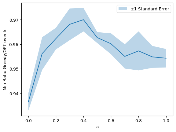
We evaluate Greedy over random graphs with left nodes whose degrees are either equal or have different level of unevenness. We use this family of instances as an example to illustrate that, for random graphs and at least experimentally, greedy seems to perform worse when the degrees of the left nodes are all equal.

To make the comparison clear, we use parameter $a\in[0,1]$ to interpolate between equal degrees ( $a=0$ ) and unequal degrees ( $a=1$ ), while keeping the average degree fixed. The instances we create for our experiments have left degrees randomly chosen from $1,4,7$ with probabilities $\frac{a}{2},1-a,\frac{a}{2}$ , so that the average degree is always $4$ . For each value of $a$ , we estimate:

\displaystyle\min_{k\in[n]}\frac{\operatorname{\mathbb{E}}\left[|N(\mathcal{G}% _{k})|\right]}{\operatorname{\mathbb{E}}\left[|N(\mathcal{O}_{k})|\right]}.

As we can see in Figure 1, the lowest ratio is achieved for equal degrees ( $a=0$ ).

Refer to caption — Figure 1: The computation is carried out for $n=m=100$ and the ratio between the value of Greedy and Opt is calculated by averaging over $50$ runs. Opt was implemented in Python using Gurobi to solve the integer program. The shaded region depicts the standard error for our estimation.

Appendix B Omitted Proofs Of Section 4

Definition 18 (Erdos-Renyi random graph).

$\mathbbm{G}_{n,m}$ samples graphs $\mathcal{G}=(V,\mathcal{E})$ , with $|V|=n$ and $\mathcal{E}\subseteq\binom{V}{2}$ chosen uniformly, such that $|\mathcal{E}|=m$ .

Definition 19 (Random graph with replacement).

$\mathbbm{G}^{r}_{n,m}$ samples graphs $\mathcal{G}^{r}=(V,\mathcal{E}^{r})$ , with $|V|=n$ . Also let $e_{1},e_{2},\dots,e_{m}\in\binom{V}{2}$ be independent uniform random samples (with replacement), then $\mathcal{E}^{r}=\{e_{1},\dots,e_{m}\}$ .

Definition 20 (Maximum matching).

Let $G=(V,E)$ and let $M$ be a maximum matching on $G$ . We denote the size of this matching as $\mu(G)=|M|$ .

Definition 21 (Maximum matching on random graphs).

Let $\mathcal{G}\sim\mathbbm{G}_{n,m}$ and $\mathcal{G}^{r}\sim\mathbbm{G}^{r}_{n,m}$ . Then $\mu(n,m)=\mu(\mathcal{G})$ denotes the size of the maximum matching on $\mathcal{G}$ and $\mu^{r}(n,m)=\mu(\mathcal{G}^{r})$ denotes the size of the maximum matching on $\mathcal{G}^{r}$ .

We state a classic result for the size of maximum matchings in random graphs by [15], but we use the statement of [3]. The difference in some constants is because we assume $n=cm$ , while in the original matching setting it was $n=cm/2$ .

Lemma 22.

[Theorem 4 in [3]] Let $n=cm$ for some constant $c>0$ and sample graph $\mathcal{G}$ from $\mathbbm{G}_{m,n}$ . Then for any constant $\epsilon>0$ we have that:

\displaystyle\Pr\left[\middle|\frac{\mu(m,n)}{m}-\left(1-\frac{\gamma^{*}+% \gamma_{*}+\gamma^{*}\gamma_{*}}{4c}\right)\middle|\geq m^{-\frac{1}{7}+% \epsilon}\right]=o(1),

where $\gamma_{*}$ is the smallest root of $x=2ce^{-2ce^{-x}}$ and $\gamma^{*}=2ce^{-\gamma_{*}}$ .

The following lemma shows that with high probability there is a sublinear number of pairs of duplicated edges in graphs drawn from model $\mathbbm{G}^{r}_{n,n}$ .

Lemma 23.

Draw $\mathcal{G}^{r}(V,\mathcal{E}^{r})\sim\mathbbm{G}^{r}_{n,n}$ . Then $\Pr\left[n-|\mathcal{E}^{r}|\geq\log{n}\right]\leq\frac{1}{\log{n}}$ .

Proof.

Let $X=n-|\mathcal{E}^{r}|$ , then $X\leq\sum_{1\leq i<j\leq n}\mathbbm{1}\{e_{i}=e_{j}\}$ , since the right-hand side counts more collisions when the same edge is sampled multiple times. Let $i\neq j$ arbitrary and we have that:

$\displaystyle\Pr\left[e_{i}=e_{j}\right]$	$\displaystyle=\sum_{\{v,v^{\prime}\}\in\binom{V}{2}}\Pr\left[e_{i}=\{v,v^{% \prime}\},e_{j}=\{v,v^{\prime}\}\right]$
	$\displaystyle=\sum_{\{v,v^{\prime}\}\in\binom{V}{2}}\Pr\left[e_{i}=\{v,v^{% \prime}\}\right]\cdot\Pr\left[e_{j}=\{v,v^{\prime}\}\right]$
	$\displaystyle=\binom{n}{2}\cdot\left(\frac{1}{\binom{n}{2}}\right)^{2}$
	$\displaystyle=\frac{1}{\binom{n}{2}},$	(1)

where the first line is by law of total probability, the second line is due to independent choice of edges and the third line is because edges are chosen uniformly at random with replacement. For the expectation of $X$ we have that:

\displaystyle\operatorname{\mathbb{E}}[X]\leq\sum_{1\leq i<j\leq n}\Pr\left[e_% {i}=e_{j}\right]=\sum_{1\leq i<j\leq n}\frac{1}{\binom{n}{2}}=\frac{\binom{n}{% 2}}{\binom{n}{2}}=1

(2)

where the second equality is by (1). Finally we show the statement:

\displaystyle\Pr\left[X\geq\log{n}\right]\leq\frac{\operatorname{\mathbb{E}}[X% ]}{\log{n}}\leq\frac{1}{\log{n}},

where the first inequality is by Markov and the second is due to (2). $\hfill\blacktriangleleft$

Now we show that the maximum matching size in both random graph models is close.

Lemma 24.

$\Pr\left[\mu^{r}(n,n)\geq x\right]\geq\Pr\left[\mu(n,n)\geq x+\log{n}\right]% \cdot\left(1-\frac{1}{\log{n}}\right)$ for all $x$ .

Proof.

We construct a coupling between $\mathbbm{G}^{r}_{n,n}$ and $\mathbbm{G}_{n,n}$ by first sampling $\hat{\mathcal{G}}^{r}=(V,\hat{\mathcal{E}}^{r})\sim\mathbbm{G}^{r}_{n,n}$ and then sampling an additional $n-|\hat{\mathcal{E}}^{r}|$ edges from $\binom{V}{2}\setminus\hat{\mathcal{E}}^{r}$ without replacement to obtain $\hat{\mathcal{G}}_{n,n}=(V,\hat{\mathcal{E}})\sim\mathbbm{G}_{n,n}$ . Then we have that:

	$\displaystyle\Pr\left[\mu^{r}(n,n)\geq x\right]$	$\displaystyle=\Pr\left[\mu(\hat{\mathcal{G}^{r}})\geq x\right]$
		$\displaystyle\geq\Pr\left[\mu(\hat{\mathcal{G}^{r}})\geq x\middle\|\|\hat{% \mathcal{E}}\setminus\hat{\mathcal{E}}^{r}\|\leq\log{n}\right]\cdot\Pr\left[\|% \hat{\mathcal{E}}\setminus\hat{\mathcal{E}}^{r}\|\leq\log{n}\right]$
		$\displaystyle\geq\Pr\left[\mu(\hat{\mathcal{G}^{r}})\geq x\middle\|\|\hat{% \mathcal{E}}\setminus\hat{\mathcal{E}}^{r}\|\leq\log{n}\right]\cdot\left(1-% \frac{1}{\log{n}}\right)$
		$\displaystyle\geq\Pr\left[\mu(\hat{\mathcal{G}})\geq x+\log{n}\middle\|\|\hat{% \mathcal{E}}\setminus\hat{\mathcal{E}}^{r}\|\leq\log{n}\right]\cdot\left(1-% \frac{1}{\log{n}}\right)$
		$\displaystyle=\Pr\left[\mu(\hat{\mathcal{G}})\geq x+\log{n}\right]\cdot\left(1% -\frac{1}{\log{n}}\right)$
		$\displaystyle=\Pr\left[\mu(n,n)\geq x+\log{n}\right]\cdot\left(1-\frac{1}{\log% {n}}\right),$

where the first line is by definition of $\hat{\mathcal{G}}^{r}$ , the second line is by law of total probability, the third line is by Lemma 23 since $|\hat{\mathcal{E}}\setminus\hat{\mathcal{E}}^{r}|=n-|\hat{\mathcal{E}}^{r}|$ , the fourth line is because conditional on $|\hat{\mathcal{E}}\setminus\hat{\mathcal{E}}^{r}|\leq\log{n}$ we have $\mu(\hat{\mathcal{G}}^{r})\geq\mu(\hat{\mathcal{G}})-\log{n}$ , so $\mu(\hat{\mathcal{G}})\geq x+\log{n}$ implies $\mu(\hat{\mathcal{G}^{r}})\geq x$ , the fifth line is due to the condition being independent of matching size $\mu(\hat{\mathcal{G}})$ and the sixth line by definition of $\hat{\mathcal{G}}$ . $\hfill\blacktriangleleft$

The following lemma gives a bound for the size of the maximum matching in graphs sampled from $\mathbbm{G}^{r}_{n,n}$ , with high probability. It is only slightly weaker than Lemma 22, which is the corresponding result for Erdős-Renyi $\mathbbm{G}_{n,n}$ . See 16

Proof.

Then we have that:

	$\displaystyle\Pr$	$\displaystyle\left[\mu(\mathcal{I}_{\mathcal{B}})\geq\left(1-\frac{\gamma^{}+% \gamma_{}+\gamma^{}\gamma_{}}{4}-n^{-\frac{1}{9}}\right)\cdot n\right]=$
		$\displaystyle=\Pr\left[\mu^{r}(n,n)\geq\left(1-\frac{\gamma^{}+\gamma_{}+% \gamma^{}\gamma_{}}{4}-n^{-\frac{1}{9}}\right)\cdot n\right]$
		$\displaystyle\geq\Pr\left[\mu(n,n)\geq\left(1-\frac{\gamma^{}+\gamma_{}+% \gamma^{}\gamma_{}}{4}-n^{-\frac{1}{9}}\right)\cdot n+\log{n}\right]\cdot% \left(1-\frac{1}{\log{n}}\right)$
		$\displaystyle=\Pr\left[\mu(n,n)-\left(1-\frac{\gamma^{}+\gamma_{}+\gamma^{}% \gamma_{}}{4}\right)n\geq\log{n}-n^{1-\frac{1}{9}}\right]\cdot\left(1-\frac{1% }{\log{n}}\right)$
		$\displaystyle\geq\Pr\left[\mu(n,n)-\left(1-\frac{\gamma^{}+\gamma_{}+\gamma^% {}\gamma_{}}{4}\right)n\geq-n^{1-\frac{1}{8}}\right]\cdot\left(1-\frac{1}{% \log{n}}\right)$
		$\displaystyle\geq\Pr\left[\big\|\mu(n,n)-\left(1-\frac{\gamma^{}+\gamma_{}+% \gamma^{}\gamma_{}}{4}\right)n\big\|\leq n^{1-\frac{1}{8}}\right]\cdot\left(1% -\frac{1}{\log{n}}\right)$
		$\displaystyle=1-\Pr\left[\big\|\frac{\mu(n,n)}{n}-\left(1-\frac{\gamma^{}+% \gamma_{}+\gamma^{}\gamma_{}}{4}\right)\big\|\geq n^{-\frac{1}{8}}\right]% \cdot\left(1-\frac{1}{\log{n}}\right)$
		$\displaystyle=1-o(1),$

the first line is by definition of $\mu^{r}(n,n)$ , the second line is due to Lemma 24, the fourth line is due to $\log{n}-n^{1-1/9}=\log{n}-n^{8/9}\leq-n^{7/8}=-n^{1-1/8}$ by the assumption for large $n$ , the fifth line is because this event is a subset, the sixth line is by taking the complement and the seventh line is due to Lemma 22 for $\epsilon=\frac{1}{7}-\frac{1}{8}>0$ . $\hfill\blacktriangleleft$

[bib.bib1] [1] Aris Anagnostopoulos, Luca Becchetti, Ilaria Bordino, Stefano Leonardi, Ida Mele, and Piotr Sankowski. Stochastic query covering for fast approximate document retrieval. ACM Trans. Inf. Syst., 33(3), 2015. doi:10.1145/2699671.

[bib.bib2] [2] Nick Arnosti. Greedy matching in bipartite random graphs. Stochastic Systems, 12(2):133–150, 2022.

[bib.bib3] [3] Jonathan Aronson, Alan Frieze, and Boris G Pittel. Maximum matchings in sparse random graphs: Karp–sipser revisited. Random Structures & Algorithms, 12(2):111–177, 1998. doi:10.1002/(SICI)1098-2418(199803)12:2\%3C111::AID-RSA1\%3E3.0.CO;2-\%23.

[bib.bib4] [4] Ricardo Baeza-Yates, Paolo Boldi, and Flavio Chierichetti. Essential web pages are easy to find. In Proceedings of the 24th International Conference on World Wide Web, WWW ’15, pages 97–107, 2015. doi:10.1145/2736277.2741100.

[bib.bib5] [5] Eric Balkanski, Sharon Qian, and Yaron Singer. Instance specific approximations for submodular maximization. In Marina Meila and Tong Zhang, editors, Proceedings of the 38th International Conference on Machine Learning, volume 139 of Proceedings of Machine Learning Research, pages 609–618. PMLR, July 2021. URL: http://proceedings.mlr.press/v139/balkanski21a.html.

[bib.bib6] [6] Joël Blot, Wenceslas Fernande de la Vega, Vangelis Th Paschos, and Rachid Saad. Average case analysis of greedy algorithms for optimisation problems on set systems. Theoretical computer science, 147(1-2):267–298, 1995. doi:10.1016/0304-3975(95)00242-O.

[bib.bib7] [7] Vaggos Chatziafratis, Tim Roughgarden, and Jan Vondrak. Stability and Recovery for Independence Systems. In 25th Annual European Symposium on Algorithms (ESA 2017), volume 87 of Leibniz International Proceedings in Informatics (LIPIcs), pages 26:1–26:15. Schloss Dagstuhl – Leibniz-Zentrum für Informatik, 2017. doi:10.4230/LIPIcs.ESA.2017.26.

[bib.bib8] [8] Michele Conforti and Gérard Cornuéjols. Submodular set functions, matroids and the greedy algorithm: tight worst-case bounds and some generalizations of the rado-edmonds theorem. Discrete applied mathematics, 7(3):251–274, 1984. doi:10.1016/0166-218X(84)90003-9.

[bib.bib9] [9] Matthias Englert, Heiko Röglin, and Berthold Vöcking. Worst case and probabilistic analysis of the 2-opt algorithm for the tsp. Algorithmica, 68(1):190–264, 2014. doi:10.1007/S00453-013-9801-4.

[bib.bib10] [10] Uriel Feige. A threshold of ln n for approximating set cover. J. ACM, 45(4):634–652, July 1998. doi:10.1145/285055.285059.

[bib.bib11] [11] W. Fernandez de la Vega, V. Th. Paschos, and R. Saad. Average case analysis of a greedy algorithm for the minimum hitting set problem. In Imre Simon, editor, LATIN ’92, pages 130–138, Berlin, Heidelberg, 1992. Springer Berlin Heidelberg.

[bib.bib12] [12] Greg N Frederickson. Probabilistic analysis for simple one-and two-dimensional bin packing algorithms. Information Processing Letters, 11(4-5):156–161, 1980. doi:10.1016/0020-0190(80)90041-1.

[bib.bib13] [13] Alan Frieze, Colin McDiarmid, and Bruce Reed. Greedy matching on the line. SIAM Journal on Computing, 19(4):666–672, 1990. doi:10.1137/0219045.

[bib.bib14] [14] Charles AR Hoare. Quicksort. The computer journal, 5(1):10–16, 1962. doi:10.1093/COMJNL/5.1.10.

[bib.bib15] [15] R. M. Karp and M. Sipser. Maximum matching in sparse random graphs. In 22nd Annual Symposium on Foundations of Computer Science (sfcs 1981), pages 364–375, 1981.

[bib.bib16] [16] Richard M Karp. Reducibility among combinatorial problems. Complexity of Computer Computations, pages 85–103, 1972. doi:10.1007/978-1-4684-2001-2_9.

[bib.bib17] [17] David Kempe, Jon Kleinberg, and Éva Tardos. Maximizing the spread of influence through a social network. In Proceedings of the Ninth ACM SIGKDD International Conference on Knowledge Discovery and Data Mining, 2003.

[bib.bib18] [18] Andreas Krause and Carlos Guestrin. Near-optimal observation selection using submodular functions. In Proceedings of the 22nd National Conference on Artificial Intelligence - Volume 2, 2007.

[bib.bib19] [19] Andrew Mastin and Patrick Jaillet. Greedy online bipartite matching on random graphs. arXiv preprint arXiv:1307.2536, 2013. arXiv:1307.2536.

[bib.bib20] [20] G. L. Nemhauser and L. A. Wolsey. Best algorithms for approximating the maximum of a submodular set function. Mathematics of Operations Research, 3(3):177–188, 1978. doi:10.1287/MOOR.3.3.177.

[bib.bib21] [21] G. L. Nemhauser, L. A. Wolsey, and M. L. Fisher. An analysis of approximations for maximizing submodular set functions – I. Mathematical Programming, 14:265–294, December 1978. doi:10.1007/BF01588971.

[bib.bib22] [22] Boris Pittel, Joel Spencer, and Nicholas Wormald. Sudden emergence of a giantk-core in a random graph. Journal of Combinatorial Theory, Series B, 67(1):111–151, 1996. doi:10.1006/JCTB.1996.0036.

[bib.bib23] [23] Sebastian Pokutta, Mohit Singh, and Alfredo Torrico. On the unreasonable effectiveness of the greedy algorithm: Greedy adapts to sharpness. In International Conference on Machine Learning, pages 7772–7782. PMLR, 2020. URL: http://proceedings.mlr.press/v119/pokutta20a.html.

[bib.bib24] [24] Aviad Rubinstein and Junyao Zhao. Budget-Smoothed Analysis for Submodular Maximization. In 13th Innovations in Theoretical Computer Science Conference (ITCS 2022), volume 215 of Leibniz International Proceedings in Informatics (LIPIcs), pages 113:1–113:23. Schloss Dagstuhl – Leibniz-Zentrum für Informatik, 2022. doi:10.4230/LIPIcs.ITCS.2022.113.

[bib.bib25] [25] Barna Saha and Lise Getoor. On maximum coverage in the streaming model & application to multi-topic blog-watch. In Proceedings of the SIAM International Conference on Data Mining, SDM 2009, April 30 - May 2, 2009, Sparks, Nevada, USA, pages 697–708. SIAM, 2009. doi:10.1137/1.9781611972795.60.

[bib.bib26] [26] Daniel A Spielman and Shang-Hua Teng. Smoothed analysis of algorithms: Why the simplex algorithm usually takes polynomial time. Journal of the ACM (JACM), 51(3):385–463, 2004. doi:10.1145/990308.990310.

[bib.bib27] [27] Satoshi Takabe, Takanori Maehara, and Koji Hukushima. Typical approximation performance for maximum coverage problem. Physical Review E, 97(2), February 2018.

[bib.bib28] [28] Orestis A Telelis and Vassilis Zissimopoulos. Absolute o(logm) error in approximating random set covering: an average case analysis. Information Processing Letters, 94(4):171–177, 2005. doi:10.1016/J.IPL.2005.02.009.

[bib.bib29] [29] Nicholas C. Wormald. Differential Equations for Random Processes and Random Graphs. The Annals of Applied Probability, 5(4):1217–1235, 1995.

[bib.bib30] [30] Nicholas C Wormald et al. The differential equation method for random graph processes and greedy algorithms. Lectures on approximation and randomized algorithms, 73(155):0943–05073, 1999.

	$\displaystyle\frac{\operatorname{\mathbb{E}}\left[\|N(\mathcal{G}_{k(n)})\|% \right]}{\operatorname{\mathbb{E}}\left[\|N(\mathcal{O}_{k(n)})\|\right]}$	$\displaystyle\leq\frac{\operatorname{\mathbb{E}}\left[\|N(\mathcal{G}_{k(n)})\|% \right]}{(1-o(1))\cdot 2k(n)}$
		$\displaystyle\leq\frac{(1+o(1))\cdot\left(\frac{1}{3}\cdot n+k(n)\right)}{(1-o% (1))\cdot 2k(n)}$
		$\displaystyle\overset{n\rightarrow\infty}{\rightarrow}\frac{1}{2}+\frac{\frac{% 1}{3}}{2-\frac{\gamma^{}+\gamma_{}+\gamma^{}\gamma_{}}{2}}$
		$\displaystyle\leq 0.94,$

	$\displaystyle\Pr$	$\displaystyle\left[\mu(\mathcal{I}_{\mathcal{B}})\geq\left(1-\frac{\gamma^{}+% \gamma_{}+\gamma^{}\gamma_{}}{4}-n^{-\frac{1}{9}}\right)\cdot n\right]=$
		$\displaystyle=\Pr\left[\mu^{r}(n,n)\geq\left(1-\frac{\gamma^{}+\gamma_{}+% \gamma^{}\gamma_{}}{4}-n^{-\frac{1}{9}}\right)\cdot n\right]$
		$\displaystyle\geq\Pr\left[\mu(n,n)\geq\left(1-\frac{\gamma^{}+\gamma_{}+% \gamma^{}\gamma_{}}{4}-n^{-\frac{1}{9}}\right)\cdot n+\log{n}\right]\cdot% \left(1-\frac{1}{\log{n}}\right)$
		$\displaystyle=\Pr\left[\mu(n,n)-\left(1-\frac{\gamma^{}+\gamma_{}+\gamma^{}% \gamma_{}}{4}\right)n\geq\log{n}-n^{1-\frac{1}{9}}\right]\cdot\left(1-\frac{1% }{\log{n}}\right)$
		$\displaystyle\geq\Pr\left[\mu(n,n)-\left(1-\frac{\gamma^{}+\gamma_{}+\gamma^% {}\gamma_{}}{4}\right)n\geq-n^{1-\frac{1}{8}}\right]\cdot\left(1-\frac{1}{% \log{n}}\right)$
		$\displaystyle\geq\Pr\left[\big\|\mu(n,n)-\left(1-\frac{\gamma^{}+\gamma_{}+% \gamma^{}\gamma_{}}{4}\right)n\big\|\leq n^{1-\frac{1}{8}}\right]\cdot\left(1% -\frac{1}{\log{n}}\right)$
		$\displaystyle=1-\Pr\left[\big\|\frac{\mu(n,n)}{n}-\left(1-\frac{\gamma^{}+% \gamma_{}+\gamma^{}\gamma_{}}{4}\right)\big\|\geq n^{-\frac{1}{8}}\right]% \cdot\left(1-\frac{1}{\log{n}}\right)$
		$\displaystyle=1-o(1),$

	$\displaystyle\operatorname{\mathbb{E}}\left[\|\mathcal{A}^{d}_{i+1}\|\!-\!\|% \mathcal{A}^{d}_{i}\|\middle\|\|\mathcal{A}^{d}_{i}\|\right]$	$\displaystyle=\Pr\left[\|N(u_{i+1})\!\setminus\!N(\mathcal{A}^{d}_{i})\|=d% \middle\|\|\mathcal{A}^{d}_{i}\|\right]$
		$\displaystyle=\frac{\binom{n-\|\mathcal{A}^{d}_{i}\|d}{d}}{\binom{n}{d}}$
		$\displaystyle\approx\left(1\!-\!\frac{d\|\mathcal{A}^{d}_{i}\|}{n}\right)^{d}$
		$\displaystyle=F\left(\frac{\|\mathcal{A}^{d}_{i}\|}{n}\right).$