The Stochastic Block Model Has the Overlap Graph Property for Modularity
 David Gamarnik
Remco van der Hofstad
Nelly Litvak
Paweł Prałat
Fiona Skerman222Corresponding author.
Yasmin Tousinejad
David Gamarnik
Remco van der Hofstad
Nelly Litvak
Paweł Prałat
Fiona Skerman222Corresponding author.
Yasmin Tousinejad
Abstract
The overlap gap property (OGP) is a statement about the geometry of near-optimal solutions. Exhibiting OGP implies failure of a class of local algorithms; and has been observed to coincide with conjectured algorithmic limits in problems with statistical computational gap.
We consider the Stochastic Block Model (SBM), where the graph has a planted partition with equal-size blocks which form the “communities”, and where, for parameters , vertices within the same community connect with probability , while vertices in different communities connect with probability , independently across pairs of vertices. Modularity–based clustering algorithms have become ubiquitous in applications. This article studies theoretical limits of local algorithms based on the modularity score on the SBM.
We establish that modularity exhibits OGP on the SBM. This rules out a class of local algorithms based on modularity for recovery in the SBM, and shows slow mixing time for a related Markov Chain. Theoretically this is one of the few instances where OGP has been established for a “planted” model, as most such analyses to date consider the “null” model.
As part of our analysis, we extend a result by Bickel and Chen 2009, who established that with high probability, the modularity optimal partition of SBM is local moves away from the planted partition, where is the graph size. We show that, with high probability, any partition with modularity score sufficiently near the optimal value is close to the planted partition.
Keywords and phrases:
community detection, average-case complexity, overlap gap property, modularity, Louvain, stochastic block modelCategory:
Track A: Algorithms, Complexity and GamesFunding:
Shankar Bhamidi: Bhamidi was partially supported by NSF DMS-2113662, DMS-2413928, DMS-2434559 and NSF RTG grant DMS-2134107.Copyright and License:
![[Uncaptioned image]](x1.png) © Shankar Bhamidi, David Gamarnik, Remco van der Hofstad, Nelly Litvak, Paweł Prałat, Fiona Skerman, and Yasmin Tousinejad; licensed under Creative Commons License CC-BY 4.0
© Shankar Bhamidi, David Gamarnik, Remco van der Hofstad, Nelly Litvak, Paweł Prałat, Fiona Skerman, and Yasmin Tousinejad; licensed under Creative Commons License CC-BY 4.0
2012 ACM Subject Classification:
Theory of computation Random network modelsAcknowledgements:
We thank Subhabrata Sen and Ekaterina Toropova for useful discussions.Funding:
This material is based upon work supported by the National Science Foundation under Grant No. DMS-1928930, while Bhamidi, Gamarnik, van der Hofstad, Litvak, Prałat and Skerman were in residence at the Simons Laufer Mathematical Sciences Institute (formerly MSRI) in Berkeley, California, during the Spring 2025 semester.Editors:
Sayan Bhattacharya, Danupon Nanongkai, Michael Benedikt, and Gabriele PuppisSeries and Publisher:
 Leibniz International Proceedings in Informatics, Schloss Dagstuhl – Leibniz-Zentrum für Informatik
1 Introduction
Modularity maximisation [28, 29] is one of the main methods used for finding clusters and communities in networks. Modularity maximisation is NP-hard [8]; in practice, modularity has a complex landscape, and there are many high scoring solutions [18]. On the other hand, one major advantage of modularity is that its local updates are easy to compute. Naturally, local updates form the initial phase in the go-to algorithms for modularity maximisation: the Louvain algorithm [6] and its improved version, the Leiden algorithm [34]. However, as already observed in [6], algorithms based on local updates get trapped in a local maximum. To avoid this, both Louvain and Leiden include an additional non-local phase. An alternative approach, proposed by Wang and Kolter [35] via the Locale algorithm, escapes local maxima by replacing the local update with low-cardinality embedding.
Given the abundance of applications of modularity maximisation and Louvain and Leiden algorithms, theoretical understanding of modularity–based algorithms is surprisingly scarce. Cohen-Addad et al. [10] proved that in the Stochastic Block Model (SBM) with sufficient signal and two equal-sized blocks, a local algorithm, very similar to the local phase of Louvain, initiated on a random bisection, recovers the correct partition with high probability. See Section 6 for further discussion including how this relates to our result.
The question remains whether local updates lead to a global optimum in this random model with more than two communities or different initialisation. In this work, we answer this question negatively. Specifically, we establish that in SBM with blocks, modularity exhibits the overlap gap property (OGP). The OGP is a statement of the geometry of near-optimal solutions and is considered a signature of algorithmic hardness – see Definition 2.1. Indeed, for many problems known to exhibit a computational-statistical gap, the threshold for OGP coincides with the conjectured algorithmic threshold [15, 16]. The idea has origins in statistical physics, and can be used to prove failure of greedy and Markov Chain Monte Carlo algorithms in average case problems. We show OGP in a planted random model as in [17, 14], though the theory is usually applied to optimisation problems in null models [15].
The practical implication of this result is that in networks with more than two communities, the local updates of Louvain or Leiden can get stuck in a local maximum even for a random graph model with clear communities. The same holds for other algorithms based on local updates. For example, Gösgens et al. [19] offer a new interpretation of modularity as an angular distance in a high-dimensional hypersphere, thus establishing equivalence of modularity maximisation and nearest-neighbour search. Then, OGP implies that greedy algorithms for nearest-neighbour search may return a local rather than the global maximum. Furthermore, using the OGP we prove that a natural generalisation of the greedy algorithm, namely the Markov Chain Monte Carlo algorithm, mixes exponentially slowly, and, in particular, takes an exponential time to reach partitions close to the planted partition with high probability.
While there are few theoretical results for modularity–based algorithms, there are positive results for recovering ground truth partitions using local-updates based on modularity in the SBM. As mentioned earlier, Cohen-Addad et al. [10] showed that for the SBM with sufficient signal and two equal-sized blocks, a local algorithm recovers the communities with high probability. This was further extended to general by giving an algorithm with parallel local updates based on the modularity function [11]. For more details and a discussion of how these relate to our OGP results, see Section 6.
More is known about the behaviour of modularity on random models; we briefly review this for context – see also the survey paper [27]. Considering first random graph models without planted structure, the main results focus on the setting of growing average degree for the random -regular graph [23, 24, 30] and the Erdős-Rényi random graph [25, 31], which are likely to have modularity of the order . For the Preferential Attachment (PA) model [2], very recently, this same behaviour was established up to log factors [32]. For models with planted structure, break-through results were given for the SBM by Bickel and Chen [4] showing that the modularity-optimal partition is close to the planted partition. These were extended to the degree-corrected SBM in [36]. See Theorem 2.4 for details. Finally, the modularity in the Artificial Benchmark for Community Detection (ABCD) model, a model similar to the well-known LFR model [21] used by practitioners, was studied in [20].
2 Results
2.1 Definitions
Let be a graph with edges and nodes. For a partition of the vertices of , the modularity score of on is defined as
| (1) |
where denotes the degree of node , denotes the number of edges within and denotes the (degree) volume of the set . The modularity of a graph is defined as , where the maximum is taken over all partitions of the nodes of . It will be useful to express modularity as the difference of the edge-contribution or coverage and the degree-tax of the partition , defined as
| (2) |
The modularity score, introduced by Newman and Girvan in [29], is a quality function of many popular community detection algorithms such as Louvain [6] or Leiden [34]. Indeed, the modularity score favours partitions of the set of nodes of a graph in which a large proportion of the edges fall entirely within the partition, but benchmarks it against the expected number of edges one would see in the same partition in a corresponding Chung-Lu random graph model [9] with expected degree sequence taken to be identical to the degree sequence of the observed graph .
Fix denoting the number of communities. We now formally define the stochastic block model (SBM) which will be the focus of this paper. This model is also called the planted partition model. The set of nodes is partitioned into communities of as equal sizes as possible; that is, for all . For simplicity, often we will assume that is divisible by , but our main result is stated and holds without this restriction. We will refer to this planted partition as . The probability of observing an edge between two nodes of the same community is equal to ; otherwise, it is equal to . We will use the notation whenever a random graph is generated with this probability distribution.
Results in the paper are in the large network limit . In particular, we will assume that both and are functions of , and is large enough for certain statements to be true. On the other hand, the parameter is an arbitrary but fixed integer. We emphasise that the notations and refer to functions of , not necessarily positive, whose growth vanishes, respectively, is bounded.

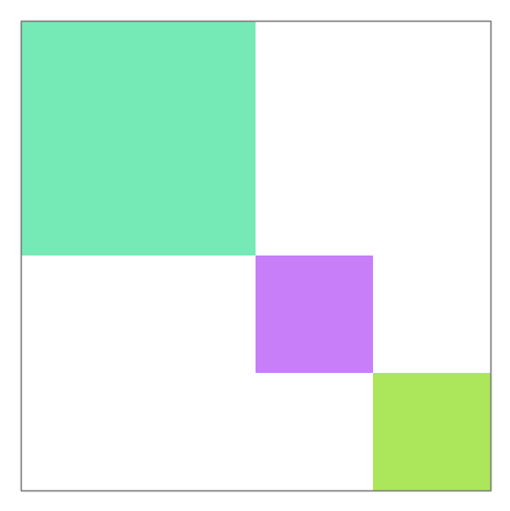
We will establish that modularity exhibits OGP in the SBM. To prove this, we will obtain a more detailed result that characterises the maximum modularity of any partition with given distance to the planted partition. We define the distance as the classification error – see, for example, (4.25) in [1]; in case of two communities, this distance is equal to the “imbalance” in [10]. Define the distance between a -part partition and the planted partition in SBM as
| (3) |
where the maximum is taken over all permutations of that govern how parts of are aligned with the ones of . Note that this has a natural interpretation: it is the minimum proportion of nodes that need to be re-shuffled to transform the candidate partition into the ground truth or planted partition . Indeed, for a given permutation , one can keep nodes in where they are and move other nodes to the appropriate parts.
Now that we have a notion of distance between partitions, we may formally define the overlap gap property (OGP). The definition of the OGP pertains to a particular instance of a distribution over graphs .
Definition 2.1 (Overlap gap property – planted model).
For a graph with planted partition , the optimisation problem exhibits OGP with values and if the following holds: For any partition for which , it holds that either , or that . Furthermore, does indeed occur for some partition with .
2.2 Modularity exhibits OGP
Theorem 2.2 below states that the modularity score exhibits OGP on the SBM, provided that the number of communities, , is at least 3:
Theorem 2.2 (Modularity has OGP).
Fix real numbers , and integer . For any and , there exist and such that the following holds for large enough.
Let and be such that , and let with planted partition . Then with probability at least , for every -part partition with
| (4) |
either or . Moreover, there are partitions satisfying the latter.
Intuition.
Consider a “decoy” partition in which two of the planted blocks are clustered together in the same part, and each of the remaining planted blocks forms its own part. (There are such decoy partitions by symmetry.) We call a “decoy” partition since it has a “misleadingly” high modularity score given its distance to the planted partition ; see Figure 1. (We emphasise that the decoy is an alternate partition of the nodes rather than an alternate random graph model to generate the graph.)
Given the decoy partition , the parameters for OGP are set as follows. We set for some small . The idea is that partitions with will include the decoy partition, those very “close to” the decoy, as well as partitions somewhat “close to” the planted (and modularity optimal) partition. Then we set for some small so that the decoy partition and those very close to it will fall within the second interval. Lastly, we need to set . Notice that, for small distances from the planted partition, the modularity score of partitions decreases with distance, so we set to be some distance by which the likely modularity score has dipped below . This explains the intuition behind Theorem 2.2.
As an implication of the OGP we show that a natural algorithm based on Markov Chain Monte Carlo (MCMC) updates takes exponential time to reach any proximity of the ground truth. We state our result informally, and defer the formal statement as well as the proof to Appendix B.
Theorem 2.3 (Informal).
For every , there exists a large enough inverse temperature parameter , such that when the chain is initiated at distance at least from the ground truth, the time to reach a partition close to the ground truth is at least with high probability.
2.3 Modularity as a predictor of the planted partition
In a breakthrough result of Bickel and Chen [4], it was shown that in the regime of growing degree, the modularity optimal partition of the stochastic block model is within distance of the planted partition (see also [5]):
Theorem 2.4 ([4, 5]).
Fix real numbers , integer and let as . Let and , and let with the planted partition . Then,
Since modularity-based clustering algorithms remain the most popular, despite known problems such as the resolution limit [13], it is reassuring that the modularity optimal partition is quite close to the “correct” partition in the SBM, a natural simplified model of community structure.
However, we would like to know more. In particular, what about partitions with nearly optimal modularity score? Are these partitions also close to the planted partition? Our Theorem 2.5 (along with some bounds on modularity scores for partitions at higher distances) implies that the answer is “yes”: if the partition has a score within a certain distance of the maximal modularity value, then the partition must be near the planted one; see the full version of the paper [3] for the proof.
Theorem 2.5 (Partitions with near-optimal modularity are close to the planted).
Fix and integer . Let and . For any and , there exists such that, if for large enough, then the following holds with probability at least provided is large enough.
Let with the planted partition . Then, for some -part partition implies that , where .
2.4 Modularity at distance at most
The next theorem relates the maximum modularity of a partition to its distance from the planted partition, and is the main ingredient in the proof of Theorem 2.2. For any , we approximate the maximum modularity value over all partitions of parts at distance (for some ) from the planted partition .
Theorem 2.6 (Maximal modularity at distance at most ).
Fix . Let and . For any , there exists such that if then the following holds with probability at least provided is large enough.
Let with the planted partition . For any , let
Then,
The random variable is defined as the maximal modularity over all -part partitions with the distance from in an interval . We keep the margins for the technical reason that there might not be any partition at distance exactly (say, when , since the distance is always a rational number). Theorem 2.6 establishes that is likely to be well approximated by the deterministic expression .
Note that function decreases on and increases on . As a result,
-
,
-
is decreasing on reaching ,
-
is increasing on reaching .
One can easily separate from its local minimum by introducing a threshold in Theorem 2.2, say, with . In Figure 2, we illustrate for and the interplay with the OGP parameters and .
Below, we will show Theorem 2.2, i.e., that modularity has OGP in the SBM – assuming Theorem 2.6, where we recall that Theorem 2.6 characterises the maximum modularity score over partitions at given distances from the planted partition . We outline the proof of Theorem 2.6 in Sections 3–5, and give some further details Appendix C. We prove Theorem 2.2 using Theorem 2.6 in Appendix D.
The asymptotic maximal modularity value in is known and also known to coincide with the modularity of the planted partition; we state it in Theorem 2.7 below for completeness. The result follows from Theorem 2.4 and was also given in [26] for slightly higher . We note that (5) in Theorem 2.7 is a direct corollary of Theorem 2.6 as a special case when . Also follows, for example, by Lemma 4.1.
Theorem 2.7 (Maximal modularity).
Fix and integer . Let and . For any , there exists such that, if for large enough, then the following holds with probability at least provided is large enough. Let and denote the planted partition by . Then,
| (5) |
and
| (6) |
As a result,
Note that, as expected, , where is defined in Theorem 2.6.
3 Ingredients of the proof : Distances to the planted partition
For now, for simplicity of exposition, we assume that is divisible by , as this will be assumed in the first lemma, Lemma 3.1. However, in the proof of Theorem 2.6, we relax this condition and deal with the general case.
To prove our main result, we need to investigate a family of partitions of with a given distance to the planted partition . It will be convenient to represent partitions as matrices that capture the way how these partitions overlap with . Let be any partition of into parts. Then, the signature of (with respect to ) is defined as the matrix , where
| (7) |
Note that for the signature to be well defined, one needs to fix the labelling of both and . To compute the distance between and , one needs to align these labels as best as possible (see Lemma 3.1 below), but the modularity score clearly does not depend on the way the labels are aligned (see Lemma 4.1 below). Note also that, trivially, for all . Moreover, since , for any ,
| (8) |
Finally, note that the signature of the planted partition is the matrix with for all and for all .
In our first lemma, we rewrite the distance between any partition and the planted partition in a convenient form, namely, as a function of the signature of . The proof is short so we give it below.
Lemma 3.1.
Suppose that is divisible by . Let be any partition of with parts, and let be the planted partition. Let be the signature of . Then,
| (9) |
where the maximum is taken over all permutations of .
Moreover, and this upper bound is sharp, that is, there exists a partition such that , provided that is divisible by .
Proof of Lemma 3.1..
Equality (9) follows immediately from the definition of the signature in (7) and the definition (3) of the distance between the two partitions. Indeed,
It remains to show that or, equivalently, that .
Consider the sum , where the outer sum is taken over all permutations of . Clearly, there are terms in and for each , the term occurs exactly times ( has to be equal to and there are permutations that map to ). Hence, for each , the sum (which is equal to 1 by (8)) occurs times. We conclude that . By an averaging argument, there exists a permutation for which . Hence, , thus the desired inequality holds.
Assume now that is not only divisible by but, in fact, it is divisible by . We construct a partition by partitioning each into equal parts and then picking fraction of each to form of size . This partition has signature with for all . We get that , which shows that the upper bound is sharp. This finishes the proof of the lemma.
4 Ingredients of the proof: Concentration
The signature of not only determines the distance between and but, more importantly, it predicts (up to an arbitrarily small error in a sufficiently dense graph ) the modularity score of for generated by the SBM. Indeed we will prove that the modularity score of is well-approximated by a scaling of , a function only of the signature of that is defined by
| (10) |
Lemma 4.1 (Concentration of modularity).
Fix and integer . Let and . For any , there exists such that if for large enough, then the following holds with probability at least provided is large enough.
Recall that the planted partition has signature with for all and for all . Since , we get that is very close to .
As one might want to use this result for other purposes, we state it (and prove it, of course) without assuming that is divisible by . The proof of Lemma 4.1 can be found in the full version of the paper [3], though we describe some intermediate steps below. One of these intermediate steps concerns the modularity score of partitions with given signature on a deterministic weighted graph. This can be regarded as a mean-field calculation. Indeed, working with the deterministic weighted graph means we may consider, for example, the edge-weight of edges in part between the planted blocks and , which corresponds to the expected number of such edges. After that step, it remains only to make a link between the modularity scores of our random graph and those of the deterministic weighted graph.
5 Ingredients of the proof: Optimisation
We have now established that, up to small errors, we may consider as our objective function, and have re-written our distance to the planted partition in terms of . Thus, the new aim is to maximise given the distance of to the planted partition .
Lemma 5.1.
Let . Define to be the family of matrices such that
| (11) | |||||
Let be defined as in (10). Then,
where, for , is the matrix with , , all other diagonal elements and non-diagonal elements (i.e., for all and for all such that ).
Note that in the optimiser , the row sums are , corresponding to part sizes in the partition at distance with (or, thus, equivalently, ).
The following lemma shows that the maximal for signatures at distance (i.e., for ) is at most the maximal for signatures at distance . This result is important to several of our proofs as it will allow us to infer that partitions with high modularity scores must be at distance from the planted partition.
The optimisation problems in Lemmas 5.1 and 5.2 are quadratic maximisation problems. (Note that in general quadratic maximisation problems are NP-hard [33].) We prove both lemmas in Appendix C. Lemma 5.1 is the last ingredient needed to prove Theorem 2.6, which gives the likely optimal modularity score over all partitions at distance from the planted partition. (Recall that we will prove our main OGP result, Theorem 2.2, in Appendix D by appealing to Theorem 2.6.) Lemma 5.2 is used to show slow mixing of a natural MCMC in Theorem B.2.
To understand how these lemmas fit in, recall that the distance to the planted partition of a partition with signature is , by Lemma 3.1 and since for each , so that . The condition corresponds to enforcing a distance of from the planted partition, and the tells us the set of partitions that achieve the maximal modularity score at distance . Note that, for , i.e. at distance of from the planted partition, is the signature for the “decoy” partition where two planted blocks and are placed within the same part, and all other planted blocks are placed within their own part – see also Figure 1.
6 Discussion and the case of optimising only over balanced partitions
The literature contains positive results, with algorithms using local updates based on the modularity function to recover communities in the SBM [10, 11]. This paper proves OGP, a signature of algorithmic hardness, for such algorithms.
Of course this does not give rise to a contradiction, since the setups in [10, 11] and ours are subtly different and also OGP has been exhibited for problems known to be easy [22]. However, it leads to interesting open questions, probing which of the differences in the two setups are important. We describe this now in more detail.
As mentioned earlier, for communities and starting with a random partition into equal-size parts, a local algorithm based on the modularity function was shown to recover the planted communities [10]. The local moves for this algorithm take the form of a swap, which takes pairs of vertices, one from each part, and swaps them if this increases the modularity score. This naturally maintains equal-size parts. For general , an algorithm with parallel local updates based on the modularity function was shown to recover the ground truth partition [11]. We note that this parallel algorithm has a random balanced start and also a mechanism to maintain the balanced sizes of parts during the algorithm.
For the overlap gap property that we establish, it was important that the “decoy” partition , which is an unbalanced partition into parts, has a “surprisingly high” modularity given its distance of from the ground truth partition . Furthermore, at distances from modularity, optimal partitions are increasingly unbalanced, with part sizes ; see Lemma 5.1.
Perhaps a crucial difference in the two setups is that the positive results of [10, 11] had balanced partitions, both in the initialisation as well as during the algorithm. We finally show that if we introduced this balanced condition into our optimisation problem then it no longer exhibits OGP. In particular, when considering where the maximisation is over balanced -part partitions instead of all -part partitions, we see that this no longer exhibits OGP. We should note that this by itself does not imply success of particular greedy algorithms – and hence fast algorithms. More work needs to be done to exhibit one (as done in [10, 11]). In a similar vain, for the problem of sparse regression [17], in the regime where OGP ceases to hold a greedy type algorithm was established to be effective. The construction is not based on OGP. Instead it relies directly on the properties of the model, which is typically the case.
To state this result, we fix the random graph under the conditions of Theorem 2.6. It turns out that the maximum modularity of only over balanced partitions at distance about from the planted partition concentrates about some function that now is decreasing in :
Proposition 6.1.
Let be defined as in (11) with the additional restriction that for all . Then is strictly decreasing on .
References
- [1] K. Avrachenkov and M. Dreveton. Statistical Analysis of Networks. Now Publishers, 2022.
- [2] A.-L. Barabási and R. Albert. Emergence of scaling in random networks. Science, 286(5439):509–512, 1999.
- [3] S. Bhamidi, D. Gamarnik, R. van der Hofstad, N. Litvak, P. Prałat, F. Skerman, and Y. Tousinejad. The stochastic block model has the overlap graph property for modularity. arXiv preprint, 2026. arXiv:2605.10911.
- [4] P. J. Bickel and A. Chen. A nonparametric view of network models and Newman–Girvan and other modularities. Proceedings of the National Academy of Sciences, 106(50), 2009.
- [5] P. J. Bickel, A. Chen, Y. Zhao, E. Levina, and J. Zhu. Correction to the proof of consistency of community detection. The Annals of Statistics, 2015.
- [6] V. D. Blondel, J.-L. Guillaume, R. Lambiotte, and E. Lefebvre. Fast unfolding of communities in large networks. Journal of Statistical Mechanics: Theory and Experiment, 2008(10):P10008, 2008.
- [7] A. Bovier and F. den Hollander. Metastability, volume 351 of Grundlehren der Mathematischen Wissenschaften [Fundamental Principles of Mathematical Sciences]. Springer, 2015. doi:10.1007/978-3-319-24777-9.
- [8] U. Brandes, D. Delling, M. Gaertler, R. Gorke, M. Hoefer, Z. Nikoloski, and D. Wagner. On modularity clustering. IEEE Transactions on Knowledge and Data Engineering, 20(2):172–188, 2007. doi:10.1109/TKDE.2007.190689.
- [9] F. R. K. Chung and L. Lu. Complex graphs and networks. American Mathematical Soc., 2006.
- [10] V. Cohen-Addad, A. Kosowski, F. Mallmann-Trenn, and D. Saulpic. On the power of Louvain in the stochastic block model. Advances in Neural Information Processing Systems, 33:4055–4066, 2020. URL: https://proceedings.neurips.cc/paper/2020/hash/29a6aa8af3c942a277478a90aa4cae21-Abstract.html.
- [11] V. Cohen-Addad, F. Mallmann-Trenn, and D. Saulpic. A massively parallel modularity-maximizing algorithm with provable guarantees. In Proceedings of the 2022 ACM Symposium on Principles of Distributed Computing, pages 356–365, 2022. doi:10.1145/3519270.3538449.
- [12] A. Coja-Oghlan, A. Galanis, L. A. Goldberg, J. B. Ravelomanana, D. Štefankovič, and E. Vigoda. Metastability of the Potts ferromagnet on random regular graphs. Comm. Math. Phys., 401(1):185–225, 2023. doi:10.1007/s00220-023-04644-6.
- [13] S. Fortunato and M. Barthelemy. Resolution limit in community detection. Proceedings of the national academy of sciences, 104(1):36–41, 2007.
- [14] D. Gamarnik. The overlap gap property: A topological barrier to optimizing over random structures. Proceedings of the National Academy of Sciences, 118(41):e2108492118, 2021.
- [15] D. Gamarnik. Turing in the shadows of Nobel and Abel: An algorithmic story behind two recent prizes. Notices of the American Mathematical Society, 72(5):485–493, 2025.
- [16] D. Gamarnik, C. Moore, and L. Zdeborová. Disordered systems insights on computational hardness. Journal of Statistical Mechanics: Theory and Experiment, 2022(11):114015, 2022. doi:10.48550/arXiv.2210.08312.
- [17] D. Gamarnik and I. Zadik. Sparse high-dimensional linear regression. Estimating squared error and a phase transition. The Annals of Statistics, 50(2):880–903, 2022.
- [18] B. Good, Y.-A. De Montjoye, and A. Clauset. Performance of modularity maximization in practical contexts. Physical Review E, 81(4):046106, 2010.
- [19] M. Gösgens, R. van der Hofstad, and N. Litvak. The hyperspherical geometry of community detection: modularity as a distance. Journal of Machine Learning Research, 24(112):1–36, 2023. URL: https://jmlr.org/papers/v24/22-0744.html.
- [20] B. Kamiński, B. Pankratz, P. Prałat, and F. Théberge. Modularity of the ABCD random graph model with community structure. Journal of Complex Networks, 10(6):cnac050, 2022. doi:10.1093/comnet/cnac050.
- [21] A. Lancichinetti, S. Fortunato, and F. Radicchi. Benchmark graphs for testing community detection algorithms. Physical Review E, 78(4):046110, 2008.
- [22] S. Li and T. Schramm. Some easy optimization problems have the overlap-gap property. In Proceedings of Thirty Eighth Conference on Learning Theory, volume 291 of Proceedings of Machine Learning Research, pages 3582–3622, 2025. URL: https://proceedings.mlr.press/v291/li25b.html.
- [23] L. Lichev and D. Mitsche. On the modularity of 3-regular random graphs and random graphs with given degree sequences. Random Structures & Algorithms, 61(4):754–802, 2022. doi:10.1002/rsa.21080.
- [24] C. McDiarmid and F. Skerman. Modularity of regular and treelike graphs. Journal of Complex Networks, 6(4):596–619, 2018. doi:10.1093/comnet/cnx046.
- [25] C. McDiarmid and F. Skerman. Modularity of Erdős-Rényi random graphs. Random Structures & Algorithms, 57(1):211–243, 2020. doi:10.1002/rsa.20910.
- [26] C. McDiarmid and F. Skerman. Modularity and partially observed graphs. arXiv preprint, 2021. doi:10.48550/arXiv.2112.13190.
- [27] C. McDiarmid and F. Skerman. Modularity and random graphs. arXiv preprint, 2025. doi:10.48550/arXiv.2509.22066.
- [28] M. E. J. Newman. Modularity and community structure in networks. Proceedings of the National Academy of Sciences, 103(23):8577–8582, 2006.
- [29] M. E. J. Newman and M. Girvan. Finding and evaluating community structure in networks. Physical Review E, 69(2):026113, 2004. doi:10.1103/physreve.69.026113.
- [30] L. O. Prokhorenkova, A. Raigorodskii, and P. Pralat. Modularity of complex networks models. Internet Mathematics, 2017.
- [31] K. Rybarczyk and M. Sulkowska. New bounds on the modularity of . arXiv preprint, 2025. arXiv:2504.16254.
- [32] K. Rybarczyk and M. Sulkowska. Modularity of Preferential Attachment Graphs. In 43rd International Symposium on Theoretical Aspects of Computer Science (STACS 2026), pages 76:1–76:19, 2026. doi:10.4230/LIPIcs.STACS.2026.76.
- [33] S. Sahni. Computationally related problems. SIAM Journal on Computing, 3(4):262–279, 1974. doi:10.1137/0203021.
- [34] V. A. Traag, L. Waltman, and N. J. Van Eck. From Louvain to Leiden: guaranteeing well-connected communities. Scientific Reports, 9(1):1–12, 2019.
- [35] P.-W. Wang and J.Z. Kolter. Community detection using fast low-cardinality semidefinite programming. Advances in Neural Information Processing Systems, 33:3374–3385, 2020. doi:10.48550/arXiv.2012.02676.
- [36] Y. Zhao, E. Levina, and J. Zhu. Consistency of community detection in networks under degree-corrected stochastic block models. The Annals of Statistics, 40(4):2266, 2012. doi:10.48550/arXiv.1110.3854.
Appendix A A guide to the proofs given in the appendix
A.1 Main results: OGP for SBM and slow-mixing
The main results in the paper are that (a) for three or more communities, the stochastic block model (SBM) exhibits the overlap gap property (OGP); and (b) failure of a natural MCMC algorithm.
For (a), that SBM exhibits OGP, the statement is Theorem 2.2, and is proven in Appendix D. Proving Theorem 2.2 requires understanding of the maximum modularity of partitions within distance of the planted partition (Theorem 2.6). Indeed, proving Theorem 2.6 is the main work of the paper, and we outline the steps in Appendix A.2.
For (b), the failure of a natural Markov Chain Monte Carlo (MCMC) algorithm, the statement is Theorem B.2 (an informal version, Theorem 2.3, appeared in the body of the paper). This algorithm is described in Appendix B, and we show in Proposition B.1 that it will likely output a partition within distance of the planted partition . However, the main result is a negative one: Theorem B.2 shows that the time taken is exponentially large in . In Appendix B, we state and prove both Theorem B.2 and Proposition B.1, assuming the OGP result stated in Theorem 2.2 and a bound on the maximum modularity of partitions at distance of the planted partition (Lemma 5.2).
A.2 Putting it all together: Proving Theorem 2.6 (which proves Theorem 2.2)
We outline the proof of Theorem 2.6; in terms of the three ingredients discussed in the main body of the paper: distances to the planted partition (Section 3), concentration (Section 4) and optimisation (Section 5).
An important definition was that of the signature of a partition ; see (7). The signature of determines the distance between and . This was established in Section 3, with all proofs contained within that section. The second and third ingredients, namely, concentration and optimisation, are more involved. The optimisation results are included in Appendix C, for the concentration results see the full version of the paper [3].
A.3 Ingredient: Concentration
We just saw that the distance of partition to the planted partition is determined by the signature of . Moreover, the signature (up to a small error) defines the modularity score of for generated by the SBM. This is established by the concentration results in Section 4 which show that for with signature , the modularity score is very close to . See (10) for a definition of . The proofs for the concentration results may be found in the full version of the paper [3].
A.4 Ingredient: Optimisation
We are interested in the maximum modularity at a given distance from the planted partition, and the concentration results tell us, loosely, that the modularity score is quite close to , where is the signature of . Hence, the remaining challenge is to understand the maximal value of over signatures of partitions at a given distance to the planted partition .
A.5 Auxiliary result: Theorem 2.5
A result of Bickel and Chen [4] states that the modularity-optimal partition is likely to be within small distance of the planted partition. We extend this to say that partitions with modularity score very close to optimal are within a small distance of the planted partition. See Theorem 2.5 for details, and the full version of the paper [3] for proofs.
A.6 Outline
We briefly outline the following sections. Appendix B proves the failure of MCMC algorithms, and Appendix C proves the optimisation results. After these sections, we prove our main result, that modularity in SBM has OGP, in Appendix D. See the full version of the paper [3] for the proofs of the concentration result Lemma 4.1, the auxiliary result Theorem 2.5, and the proof Proposition 6.1 which concerns the setting in which we restrict to optimising only over balanced partitions.
Appendix B Failure of the Markov Chain Monte Carlo algorithm
Throughout this section we consider -partitions with fixed. We denote , for brevity. The OGP immediately implies the failure of a natural Greedy algorithm for finding the planted partition when started from the decoy partition . More specifically, Greedy is an algorithm resulting in a sequence of partitions built as follows: We initialise the Greedy algorithm in the decoy partition, i.e., . Given , the partition is obtained by changing the membership of at most one node such that the resulting modularity strictly increases. That is, is any partition satisfying and . If no such node exists, then the algorithm stops and outputs the partition obtained in the final step. By the OGP, the Greedy algorithm, initiated at the decoy partition , terminates at this partition with distance at least from the ground truth.
A natural generalisation of the Greedy algorithm, which is guaranteed (as we will show) to output a partition approximately matching the planted partition , is the well-known Markov Chain Monte Carlo (MCMC) algorithm which we now describe. Our main result in this section is the proof of slow mixing of this MCMC. In particular, we will show that the time it takes for the algorithm to approximately produce an planted partition is exponentially large in .
We begin by describing the MCMC algorithm. A parameter usually called the inverse temperature is fixed. The algorithm proceeds as a Markov chain moving according to the following rules. Given any partition , consider any partition with . Then the algorithm moves from to with probability proportional to , namely with probability
where here the sum is over all partitions with . (Note that we choose this parametrisation so that the stationary distribution is informative.) It is known that the unique stationary distribution of this chain is the so-called Gibbs distribution given by
where is the normalising constant, which is also called the partition function, and now the sum is over all partitions .
We first show that this algorithm is sound, in the sense that for large enough it produces partitions that are close to the ground truth .
Proposition B.1.
For every , there exists large enough such that
In words, the probability mass of partitions with distance at most from the planted partition constitutes at least a fraction of the total probability mass. Thus, if the algorithm were to run until stationarity, then a partition sampled according to the Gibbs distribution is likely to be at most close to the ground truth, modulo an at most likelihood event.
Proof of Proposition B.1.
Given any let . Fix . By Theorem 2.5, we can find small enough so that, with probability at least , the event occurs that every satisfying satisfies . On this event,
Fix large enough so that (any strictly negative constant will do). Then, this sum is at most , so that
for large enough . Combining this event with the complement event, which occurs with probability at most , we complete the proof.
Our main result, described next, shows that unfortunately the time to stationarity is exponentially large in when the chain is initiated at a large enough distance from the partition, appropriately defined. Worse than that, the time to reach even one partition close to the ground truth is exponentially large in , again when the chain is initiated at a large distance from the ground truth. This means that the set of such starting points acts as a metastable set. See [7] for a discussion on metastability, and [12] for an example of metastability in random regular graphs.
In preparation for the proof of this claim, we recap some of the properties implied by the OGP and an auxiliary lemma: there exist and such that the following holds. Let
Then, by Theorem 2.2 and Lemma 5.2 with probability at least
| (12) | |||
| (13) | |||
| (14) |
We now state our lower bound result.
Theorem B.2.
Consider the MCMC initiated at the Gibbs distribution conditioned on being in . Namely, suppose
for all , and otherwise. Let . There exist such that with probability at least (with respect to the randomness of the graph)
where the probability is with respect to the random choices of the MCMC.
Proof.
We assume that the events (12)-(14) hold, which is the case with probability at least . We note that the events imply the existence of such that . For every positive integer ,
We have
Thus the ratio is at most . Assuming is large enough so that (again any negative constant suffices), this ratio is at most . By the union bound, we obtain that , completing the proof.
Appendix C Optimisation lemmas for modularity at a given distance
In this section we prove that the function has the required behaviour. Recall that by Theorem 2.6 with probability close to one, the modularity of any partition with signature can be well approximated by .
In particular, we are interested in the maximum modularity score for partitions at a given distance ; and this we can control by understanding the maximum of for signatures at distance ; or, equivalently, the maximum of , which we call . (See also the discussion after Theorem 2.6.) This will correspond to the maximisation problem for the -block SBM, and re-scaled distance .
These results naturally split into two. For , we solve this optimisation in Lemma 5.1, while, for , we show in Lemma 5.2 that , i.e., that the value of is bounded above by its maximum at .
C.1 Proof of the general case for distance
Proof of Lemma 5.1.
Let and consider first . We will prove the result by successively eliminating the variables.
We begin by giving an equivalent optimisation problem with variables. Since the columns of the matrix sum to , we may reduce the number of variables by writing , and maximising the resulting obtained from by making these substitutions for .
In particular, let
| (15) |
Thus it will suffice to show has the bounds claimed. (We write , since we have now a subset of variables of the matrix .)
Notice that if we have equality for for some all distinct, then , which yields a contradiction since . Thus, it is equivalent to consider the maximisation problem over , where we require strict inequality for the terms, i.e., . Let
| (16) |
It now suffices to show that satisfies the claimed bounds.
We may remove one more variable. Note from the constraints that we have
Let be making this substitution (i.e., is a function on variables), and let
| (17) | |||||
Thus, finally, it suffices to show that satisfies the claimed bounds.
Recall that the maximum of a convex function is obtained on the boundary. Note also that we may apply this recursively, since if we set any inequality in (17) to equality, then we may make a substitution to reduce the number of variables by , and we obtain a maximisation problem for a convex function (on one fewer variables). Thus, the max of over is obtained when at least of the inequalities in (17) are equality.
Observe that there are inequalities in (17) (which are not strict inequalities), so the maximum is obtained when we set all but (at most) one of these to equality.
We consider two cases. The first case is that we have for all with . Notice that this fixes the value of all variables, and that the remaining inequalities in (17) are all satisfied. The value of attained is that of with (and for all with , and for all ). Note that this yields the matrix , and, moreover, that .
The second case is that there exist (where ) such that
Notice that this fixes the value of all variables: and all remaining variables take the value , and that this assignment satisfies the remaining inequalities in (17). The value of , attained is that of with (and for all with , and for all ). Note that this yields the matrix , and, moreover, that again for any such . This completes the proof.
C.2 Proof for the general case
Here we prove Lemma 5.2, which will allow us to infer that partitions with high modularity scores must be at distance from the planted partition.
Proof.
Consider any partition with signature that is at distance more than from the planted partition . Our goal is to show that .
Suppose that there exists a column (say, ) in with at least two non-zero entries (say, and ). Consider a family of signatures that is parametrised by variable , as follows: for a given , matrix is exactly the same as but is replaced with and is replaced with . Of course, .
Note that is a quadratic function of with a positive coefficient in front of . As a result, at least one of the following two properties holds: (i) increases as increases from to (which is equivalent to transferring a weight from to ); or (ii) increases as decreases from to (which is equivalent to transferring a weight from to ). Note that it might be the case that attains its local minimum at and both properties hold at the same time. Regardless, we may start from and either increase or decrease to gradually increase . While we do this, the distance to the planted partition does not need to behave monotonically. However, it is easy to see (but it is crucial for the argument) that the distance to is a continuous function of . Once we are done with transferring the weight, we get an additional zero entry in our signature matrix, and we can move on to the next pair of non-zero entries, possibly in a different column .
We need to consider two cases now. Suppose first that during the above process the distance to is equal to . We prematurely stop the process at the very first time this happens, and let be the signature we have at that moment. Since we kept increasing the function along the way, it follows from Lemma 5.1 (applied with ) that
which finishes the proof of the lemma in this case.
Suppose now that the distance from to was always more than , but we had to stop the above process of transferring weights at some point because each column had exactly one non-zero entry (of course these non-zero entries must be equal to one). This means that each part of is a union of some planted parts, and the distance between and is equal to for some integer .
Now, take any part which is a union of planted parts and split it into two parts, consisting of and a single planted part, respectively. After such partition refinement, the function increases. Indeed, before splitting the part with planted parts, the contribution of that part to the function is , but after splitting, the two resulting parts contribute , which is equal to . We continue such refinements of partitions until the distance to is . At that point, the partition with signature has one part consisting of two planted parts, while the remaining parts consist of just one planted part. The conclusion is as before:
This finishes the proof of Lemma 5.2.
Appendix D Proof of Theorem 2.2: SBM has OGP
Proof of Theorem 2.2.
We will prove Theorem 2.2 using Theorem 2.6, our concentration result in Lemma 4.1, and the optimisation result in Lemma 5.2.
First, we will set up the range for the distances. Recall that is a quadratic function of , with minimum at . See also Figure 2. Take any , choose , and let be the unique number such that . Let be the smallest integer such that .
Next, we define . Choose a positive . Then, by Theorem 2.6, we obtain that parts (i) and (ii) below hold with probability at least , and for large enough:
-
1.
For all partitions at distance and at distance , it holds that
-
2.
For any partition at distance ,
Together, the above establish Theorem 2.2.