Near-Optimal Dynamic Data Structures for Maximum Depth and Klee’s Measure of Boxes

Abstract
We study two fundamental geometric problems on a dynamic set of axis-parallel boxes in -dimensional space. The maximum depth problem asks for the largest number of boxes that contain a common point, whereas Klee’s measure problem asks for the volume of the union of the boxes. We present fully dynamic exact data structures for both problems achieving amortized update time. This update time is optimal for an exact dynamic algorithm, up to logarithmic factors, assuming the Combinatorial -Clique Hypothesis. Previously, matching bounds were established only for [Imai and Asano, J. Algo.’83], and for [Suri, Xue, Yang, and Zhu, SoCG’25].
Our approach integrates a classic grid-based partition framework with a novel charging analysis that controls the cost of structure-sensitive offline routines within each cell. This argument allows us to perform a global aggregation of the update time, by circumventing the worst-case costs associated with individual cell updates. We believe this technique may be of independent interest for other dynamic geometric problems.
Keywords and phrases:
dynamic algorithms, maximum depthCategory:
Track A: Algorithms, Complexity and GamesCopyright and License:
![[Uncaptioned image]](x1.png) © Sujoy Bhore, Subhash Suri, Jie Xue, Xiongxin Yang, and Jiumu Zhu; licensed under Creative Commons License CC-BY 4.0
© Sujoy Bhore, Subhash Suri, Jie Xue, Xiongxin Yang, and Jiumu Zhu; licensed under Creative Commons License CC-BY 4.0
2012 ACM Subject Classification:
Theory of computation Design and analysis of algorithmsEditors:
Sayan Bhattacharya, Danupon Nanongkai, Michael Benedikt, and Gabriele PuppisSeries and Publisher:
 Leibniz International Proceedings in Informatics, Schloss Dagstuhl – Leibniz-Zentrum für Informatik
1 Introduction
For a set of geometric objects, the maximum depth of is the largest number of objects in that have a nonempty common intersection. Maximum depth is an important parameter capturing the local density of a family of geometric objects, and it has appeared in many geometric and combinatorial settings. The maximum depth is closely related to the clique number of the intersection graph of the objects. For example, for families with Helly number two – including axis-parallel rectangles and boxes – pairwise intersection implies a nonempty common intersection, and thus the maximum depth is exactly the size of a maximum clique in the corresponding intersection graph [19, 26]. For fat objects in fixed dimension, the maximum depth still provides a constant-factor approximation to the maximum clique size of the intersection graph.
Computing the maximum depth of an input family of objects in is a fundamental problem in computational geometry and has been studied since the early days of the field [24, 18, 4, 1, 3, 13, 30]. For (axis-parallel) boxes in , the maximum depth problem can be solved in time [29, 12, 13]. This bound is believed to be tight up to logarithmic factors, since any improvement would break the Combinatorial -Clique Hypothesis [12].
For boxes, a closely related problem is Klee’s measure: given a set of boxes, compute the volume of their union (the Klee’s measure of ). The problem was first posed in 1977 by Klee [25], and it is among the earliest questions that influenced the development of computational geometry. Since then, it has been studied extensively [6, 31, 29, 12, 13, 5]. Moreover, algorithms for Klee’s measure can typically be adapted to solve the maximum depth problem with essentially the same running time [5]. In 1991, Overmars and Yap [29] gave the first -time algorithm for Klee’s measure in . About two decades later, Chan [12, 13] simplified and refined the approach to obtain an -time algorithm. Again, this bound is conditional tight up to logarithmic factors [12].
In this paper, we study the dynamic versions of the maximum depth problem and Klee’s measure problem for boxes in . In this fully dynamic setting, boxes may be inserted and deleted over time, and the goal is to maintain the maximum depth (respectively, Klee’s measure) of the current set efficiently. Since the seminal work of Overmars and van Leeuwen [28], dynamic geometric data structures have played a central role in computational geometry. Many classic geometric problems have been studied extensively in the dynamic model, leading to a rich collection of efficient data structures, including convex hulls [23, 10], closest pairs [20, 21, 14], range searching [27, 17], geometric width [11], geometric set cover and hitting set [15, 2, 16], geometric independent set [22, 9, 7], and geometric vertex cover and matching [8], among others. Due to the importance of maximum depth and Klee’s measure, it is natural to ask how efficiently one can maintain these quantities for a dynamic set of boxes in .
The near-optimal running time for the static problems yields a lower bound for the dynamic setting via a standard sweep-line reduction: Given a dynamic data structure for maximum depth (or Klee’s measure) for boxes in with update time , one can obtain a static algorithm for boxes in with running time by applying the sweep-line framework of Imai and Asano [24]. Consequently, a dynamic data structure in with update time would yield a static algorithm in with running time . In light of this reduction, the most compelling goal is to design dynamic data structures whose update time matches the barrier up to logarithmic factors. We formulate this as the following question, which is the main focus of this paper.
Do there exist dynamic data structures for maximum depth and Klee’s measure of
axis-parallel boxes in with update time ?
For , the classic work of Imai and Asano [24] achieves update time and thus answers the above question affirmatively. Beyond this base case, however, the question had remained poorly understood. Only very recently, Suri, Xue, Yang, and Zhu [30] proposed (among other results) a dynamic maximum-depth data structure for rectangles in the plane with amortized update time. With additional work, their ideas can be adapted to maintain Klee’s measure for planar rectangles as well, yielding update time. This resolves the above question for . Unfortunately, while the 2D framework [30] extends to higher dimensions, it does not achieve the target bound of , already for (see discussion in Section 2). Prior to this work, the above question was open for any value of .
The main contribution of this paper is to answer the question in the affirmative for every fixed . Specifically, we design fully dynamic data structures for both maximum depth and Klee’s measure of axis-parallel boxes in with update time.
Theorem 1.
There exists a fully dynamic maximum depth data structure for axis-parallel boxes in with amortized update time.
Our techniques extend beyond depth queries and also yield an efficient dynamic structure for maintaining the union volume for boxes.
Theorem 2.
There exists a fully dynamic Klee’s measure data structure for axis-parallel boxes in with amortized update time.
2 Technical Overview
We provide an overview of our fully dynamic maximum-depth data structure. We focus on the high-level ideas and the role of the key charging quantities. The dynamic Klee’s measure structure follows the similar framework with a different interval primitive.
2.1 Overview of the 2D data structure
We start by recalling the main idea behind the 2D data structure of [30]. It partitions the plane into vertical strips so that each strip contains rectangle corners, and maintains the maximum depth inside each strip separately. Although rectangles may intersect a fixed strip, all but of them have no corner in it; we call these rectangles good (for the strip), and the remaining rectangles bad. Inside the strip, every good rectangle spans the strip in the -direction and is therefore equivalent to an interval on the -axis. This reduces the subproblem inside the strip to maintaining the maximum depth of a dynamic set of (weighted) intervals: updates caused by good rectangles take only time, while updates caused by bad rectangles take time, since there are only bad rectangles whose contribution must be recomputed. Moreover, each rectangle is bad for only strips (namely those containing its left or right vertical side), and is good for all other strips. Overall, the update time is , which becomes by setting .
2.2 Challenges in higher dimensions
A natural goal in is to replicate the same high-level principle: partition space so that most boxes behave “one-dimensionally” inside each region (and can be maintained cheaply), while only a small set of boxes interacts with the region boundaries. Two straightforward generalizations break down for essentially the same reason: the contribution of the boundary-interacting (“bad”) boxes can have prohibitively large combinatorial complexity. There are multiple natural generalizations of this approach to higher dimensions; however, none of them guarantees the desired bounds.
-
Partition into slabs along one axis: Partition into slab regions perpendicular to the -axis, each containing box corners. Inside a slab , good boxes are those with no corner in ; they span the slab in the -direction and thus reduce to -dimensional boxes via projection. The difficulty is with the bad boxes: their contribution inside can be described by a piecewise-constant depth function over whose rectilinear decomposition may require regions in the worst case (because arrangements of boxes in can have complexity ). Thus, even assuming optimal lower-dimensional dynamic structures, the induced subproblem sizes are too large to support the target update time.
-
Partition into cells in the first dimensions: Choose hyperplanes perpendicular to each of the first coordinate axes, so that these hyperplanes form a grid partition of into cells, each of the form , where is a -dimensional axis-parallel box. Inside a fixed cell , a box is good if it spans the cell in the first coordinates, i.e., it completely covers . Restricted to the cell, such a box contributes exactly one interval on the last axis and can be maintained with a dynamic maximum-depth data structure for intervals. The bottleneck is the remaining bad boxes, namely those that intersect but do not cover it, so some side facet of the box crosses the base . A direct adaptation would handle these bad boxes in each affected cell by sweeping along the last axis and repeatedly invoking a -dimensional dynamic maximum-depth subroutine. Even assuming optimal lower-dimensional update bounds, this becomes too expensive once summed over the cells whose bases can be intersected by the boundary of a single updated box.
2.3 Overview of Our Techniques
At a high-level, we also follow the grid partition into cells of the form , and we retain the same “good boxes interval updates” principle. The key new ingredient is a structure-sensitive way to process the bad boxes within a fixed cell.
Fix a cell , and consider the set of bad boxes whose projections intersect but do not cover it. Our data structure represents their contribution to the depth inside by a piecewise-constant function on the last coordinate (equivalently, by a set of weighted (type-2) intervals, one per piece). Thus, for a cell , the total depth reduces to the maximum depth of a set of weighted intervals on the last axis: type-1 intervals coming from good boxes (weight ) plus the type-2 intervals capturing the bad-box contribution.
The core task in an update is therefore the following: when the bad-box set for a cell changes, we must recompute the new inside- depth function (and hence the new set of type-2 intervals) efficiently. We accomplish this via an offline subroutine that further refines by inserting additional axis-parallel hyperplanes so that, inside every resulting subcell, each bad box becomes equivalent to a slab in (i.e., it is bounded in exactly one of the first directions and is either fully present or fully absent in the other directions throughout the subcell). Once this holds, the contribution of the bad boxes inside each subcell reduces to a one-dimensional interval problem on the last axis.
The key idea to keep the refinement small is to avoid cutting at every bad-box endpoint in every partially overlapping direction. Instead, we choose an ordering (permutation) of the first coordinate axes. For a given bad box, we treat the earliest axis (in -order) along which it only partially overlaps as its active direction (the slab direction), and we cut at the box endpoints only in the later partially overlapping directions. Equivalently, the box charges every partially overlapping direction except its first one under . In the formal development, this choice is captured by the indicators and the counts . For a fixed , the number of inserted hyperplanes perpendicular to axis is proportional to , and the number of resulting subcells is bounded by , which also governs the running time of the offline subroutine.
In the dynamic data structure, we maintain the values for every cell , every axis , and every permutation . When an update changes the bad-box set in a cell, we pick the permutation that minimizes the product bound and invoke the offline subroutine under this choice to compute the updated inside- depth function (and hence the new type-2 intervals) for that cell. Meanwhile, updates from good boxes remain fast interval insertions/deletions (type-1 updates).
The remaining challenge is to argue that the total cost of these offline computations over all cells affected by a single box update is bounded by . This is where the main charging analysis enters. The affected cells lie on “slices” of the grid determined by the facets of the projected box: fixing a coordinate and a slab index specifies a family of cells . A global charging argument relates each local quantity to the distribution of box corners among these slices and shows that, for any slice , choosing an order whose first element is yields a strong bound on (Lemma 11). Combining this with the fact that each affected cell contains only bad boxes yields the desired amortized update time after setting .
3 Preliminaries
Basic Notations.
We use to denote the set of positive integers and define . For an integer , we write . Throughout the paper, all rectangles and boxes are axis-parallel.
Projection.
Let be a box in . For , let denote the interval obtained by projecting onto dimension . More generally, for where , let denote the -dimensional box obtained by projecting onto the dimensions in . For a set of boxes in , we write for and for .
Maximum depth.
Let be a set of geometric objects in . For a point , we define , which is called the depth of at . For a region , we define , which is called the maximum depth of inside . We write for the maximum depth of .
Klee’s measure.
For a geometric object in , we denote by the volume of . Let be a set of geometric objects in . For a region , we define , which is called the Klee’s measure of inside . We write for the Klee’s measure of . Note that can be if contains unbounded objects.
Piecewise constant functions.
We say that a function is piecewise constant if can be partitioned into finitely many intervals such that, for every , the restriction is constant. Such a partition need not be unique. If we require to be minimum possible, then the resulting partition into maximal intervals on which is constant is uniquely determined; we call these intervals the pieces of and denote them by . For each piece , we write for an arbitrary ; this value is well-defined since is constant.
4 Offline dynamic maximum depth
In this section, we consider an offline variant of the dynamic maximum depth problem and propose an algorithm whose running time depends not only on the number of update operations but also on the structure of the boxes involved. We will use this offline algorithm as a subroutine in our fully dynamic data structure.
Offline Inside- Box Maximum Depth in
Input: An initially empty set of boxes in , a fixed box region , and a sequence of updates to , each of which is of one of the following two types:
-
Insertion: Insert a new box into .
-
Deletion: Delete an existing box from
Output: A sequence , where is the maximum depth of inside the region after the -th update.
4.1 Dynamic maximum depth for slabs
In designing our algorithm, we require an efficient dynamic maximum-depth data structure for slabs, i.e., boxes that are bounded in exactly one dimension. Formally, a slab in is a box such that there exists exactly one index satisfying .
If we have a dynamic set of slabs in that are all bounded in the same dimension, then maintaining the maximum depth of reduces to maintaining the maximum depth of a dynamic set of intervals and can be done with logarithmic update time. Moreover, the following observation implies that even if the slabs in are bounded in different dimensions, we can still maintain the maximum depth of with logarithmic update time by handling each dimension separately.
Fact 3.
Let be a set of slabs in and be a fixed box in . Then we have , where consists of the slabs bounded in dimension .
Proof.
Since , we have . It remains to show the reverse inequality. For each , let be a point satisfying . Since all slabs in are perpendicular to the -axis, we have for any point whose -th coordinate is equal to that of . Let denote the point whose -th coordinate equals the -th coordinate of for every . Then for all , and thus
Moreover, since . Therefore, .
Lemma 4.
Let be a fixed box in . There exists a dynamic inside- maximum depth data structure for slabs in with update time.
Proof.
Let be a dynamic set of slabs in , and for each let denote the slabs perpendicular to the -axis. For each , we maintain a data structure that supports updates to and maintains . Maintaining reduces to the one-dimensional problem of maintaining the maximum depth of the dynamic interval set inside the interval , which admits update time [24]. An insertion or deletion of a slab affects exactly one index , and thus triggers a single update to the corresponding . Therefore, by Fact 3, together maintain . The update time is .
4.2 Solving the offline problem
Let be a box in . We say a box in is nontrivial in dimension with respect to if and . For a permutation of , an index , and a box in , we define if both of the following conditions hold:
-
is nontrivial in dimension with respect to ,
-
there exists such that is nontrivial in dimension with respect to .
Otherwise, . For a set of boxes in , define .
Lemma 5.
Let be a permutation of and be a fixed box in . Then Offline Inside- Box Maximum Depth in can be solved in time, where denotes the set of all boxes that are inserted into in the sequence of updates.
Proof.
For simplicity, we present the proof for the case and drop the subscript in the notation. the argument extends verbatim to an arbitrary fixed box by restricting attention to . Without loss of generality, we assume the boxes in are in general position in the sense that, for every , the intervals in have distinct endpoints.
For each , we define a set of hyperplanes perpendicular to the -axis as follows. Let . For each endpoint of each interval in , we include in the hyperplane . Note that . The hyperplanes in partition the space into cells; let denote the resulting set of cells. For each cell , we maintain a dynamic data structure that maintains the maximum depth of the current set inside the interior of ; denote this value by . Under the general-position assumption, the maximum depth of is attained in the interior of some cell, and thus equals . Therefore, replaying the updates for every yields a total running time , where is the maximum update time of each individual .
The remaining task is to achieve . The key observation is that, inside the interior of any fixed cell , every box behaves like a slab. To see this, fix and suppose is nontrivial in dimensions with respect to , where . By the definition of , we have . Hence, for each , we added to the two hyperplanes corresponding to the endpoints of . It follows that, for each such , the interior of is either contained in or disjoint from it. Therefore, inside the interior of , the box has the same intersection as the slab . As a consequence, inside the interior of , maintaining the maximum depth of reduces to maintaining the maximum depth of a dynamic set of slabs. We can therefore instantiate using Lemma 4, which supports updates in time. This gives and yields a total running time as claimed.
Let be a region in and let be a set of boxes in . We define the inside- depth function of as the function given by for all . Note that is a piecewise constant function, for any choice of . Indeed, as moves from to , the set of boxes intersecting the slice can change only when reaches an endpoint of an interval in . Our offline algorithm above directly implies an algorithm for computing the inside- depth function for a fixed box , which will be used in our dynamic data structure.
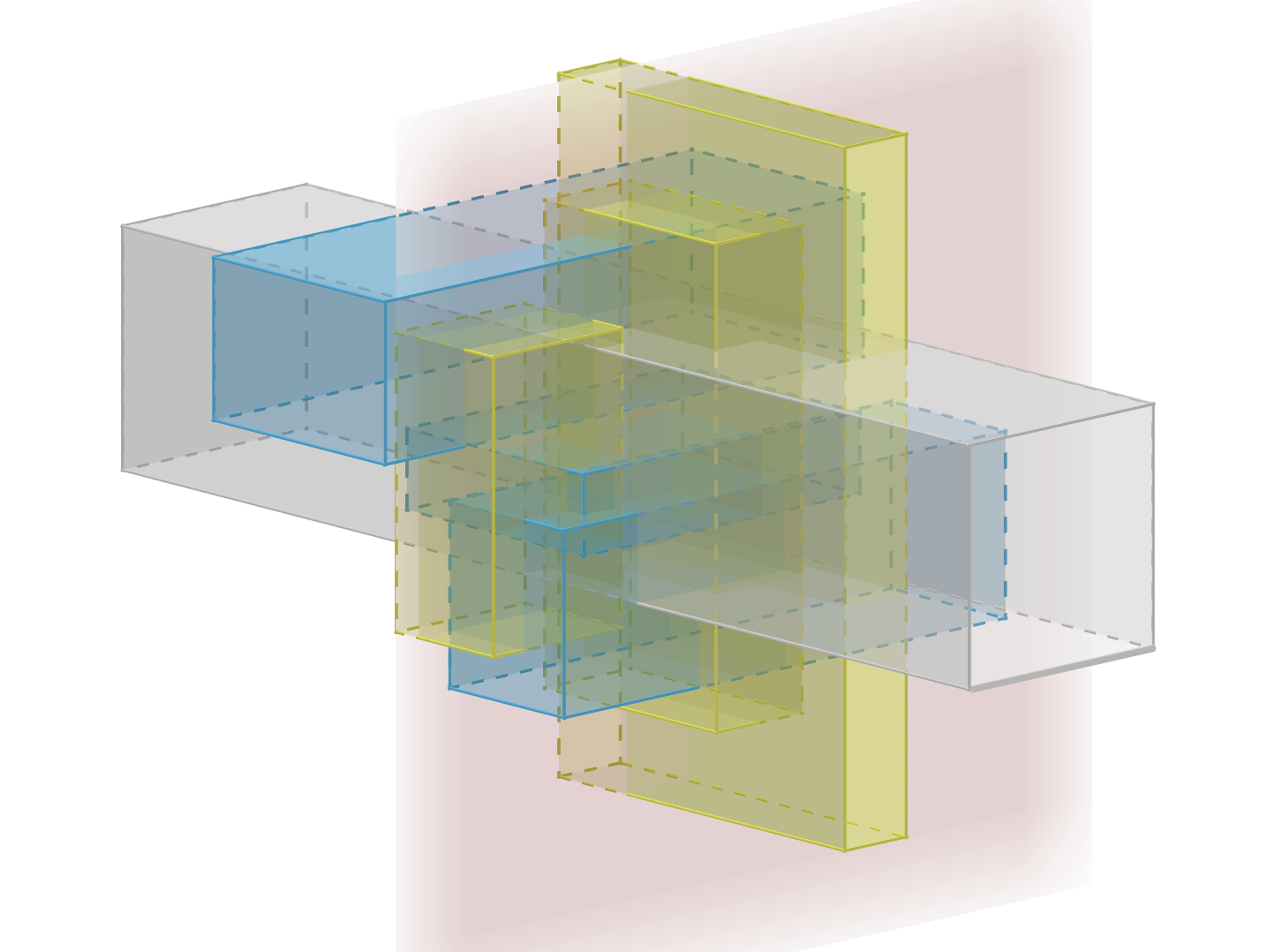
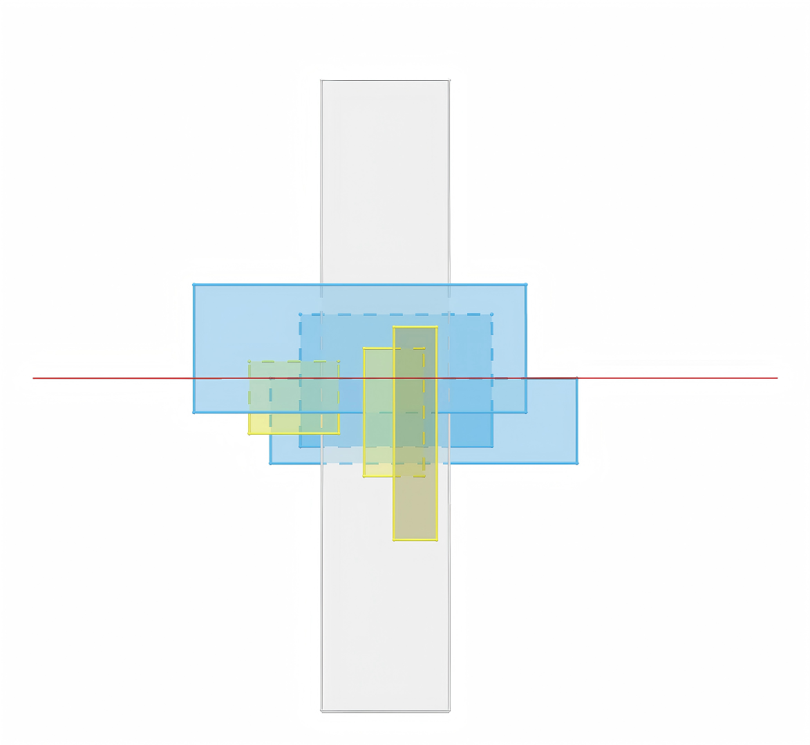
Corollary 6.
Given a permutation of , a box in , and a set of boxes in , one can compute the inside- depth function in time.
Proof.
Let be the set of endpoints of the intervals in . Without loss of generality, assume that the boxes in are in general position, so contains exactly distinct points with . Consider a point moving from to on -axis, and maintain a dynamic set of boxes in , initially empty. Whenever reaches a point , if is the left (resp., right) endpoint of for some , then we insert into (resp., delete from ) the box . Clearly, for any , equals the maximum depth of inside at the time . Thus, to compute , it suffices to maintain the maximum depth of inside under this sequence of insertions and deletions. This is an instance of Offline Inside- Box Maximum Depth in , as the update sequence is fully known in advance. Moreover, the set of boxes that are ever inserted into is exactly . Applying Lemma 5 completes the proof and yields the stated running time .
5 Dynamic data structure for maximum depth
We now describe our dynamic data structure for maintaining the maximum depth of a dynamic set of boxes. Let be a dynamic set of boxes in , which contains boxes initially. Let be a parameter to be specified later.
5.1 Construction of the data structure
In the preprocessing, for each dimension , we construct a set of hyperplanes in perpendicular to the -axis such that, after sorting the hyperplanes along the -axis, the number of corners of boxes in lying between any two consecutive hyperplanes is . Let . The hyperplanes in partition into regions, which we call cells. We index cells by vectors , where indicates the position of the cell along dimension (i.e., the cell lies between the -st and -th hyperplanes in , with the two outermost slabs treated as unbounded). Since we do not introduce hyperplanes perpendicular to the -axis, each cell is of the form for a box . For each , let denote the unique box in such that the corresponding cell is .
By the standard periodic reconstruction trick, we may assume that throughout the reconstruction period. For simplicity, we also assume that, throughout the period, for each , the number of corners of boxes in between any two consecutive hyperplanes in remains . This assumption can be removed by applying the same splitting procedure as in [30]; we defer these implementation details to Appendix A.
For each , our data structure maintains the following information:
-
for all permutations of and all .
-
The subset .
-
A dynamic maximum-depth data structure for weighted intervals, storing a multiset that consists of:
-
–
the interval with weight , for every with ; these are called type-1 intervals,
-
–
the interval with weight , for every piece of the function ; these are called type-2 intervals.
-
–
The basic correspondence between and the inside- depth function is easy to establish.
Observation 7.
for all .
Proof.
Fix . By construction, equals plus the number of boxes satisfying and . The latter quantity is exactly . Therefore, . The intervals in are stored in the data structure for weighted intervals. Observation 7 implies that , and hence . Accordingly, maintaining the values and taking their maximum over all suffices to obtain .
Consider an update on a box that either inserts into or deletes an existing box . We process the update for every . First, we update the values for all permutations of and all . This is straightforward: for each such pair , we compute and either add it to or subtract it from the current value of , depending on whether the update is an insertion or a deletion. We then update the set , which is also immediate from its definition.
Next, we update the data structure , since the interval multiset may change. There are three cases. If , then does not change. If , then changes only by a single type-1 interval: we insert (with weight ) if is inserted, or delete the corresponding type-1 interval if is deleted. Thus, it suffices to perform one insertion/deletion operation in .
In the remaining case, we have and , i.e., . In this case, the type-2 intervals in change, and we proceed as follows.
-
1.
Pick a permutation of that minimizes .
-
2.
Apply the algorithm of Corollary 6 with this permutation to compute the updated inside- depth function , which in turn specifies the updated set of type-2 intervals in .
-
3.
Delete the old type-2 intervals from and insert the new type-2 intervals into .
We perform the above update for all . Correctness follows from Observation 7 and the fact that always stores exactly the current interval multiset . The main challenge is to prove that this procedure achieves the desired amortized update time .
5.2 Update time analysis
We show that each update of our data structure can be processed in time. Setting then yields the desired bound .
Consider an update that inserts a new box or deletes an existing box . First observe that, for every such that does not change, the corresponding local update costs only time (it consists of maintaining counters and possibly inserting/deleting a single type-1 interval). In total, this contributes time. It therefore suffices to focus on those for which changes; let denote this set. Note that consists exactly of the vectors for which intersects the boundary of . For , all steps of the update can still be performed in time except: (i) recomputing via Corollary 6, and (ii) deleting the old type-2 intervals from and inserting the new ones. Since has pieces, step (ii) costs time, which is dominated (up to logarithmic factors) by the cost of step (i). Thus, it suffices to bound the total cost of computing for all .
Let denote the set of boxes after the insertion/deletion of . For and , define
Intuitively, the cells with are precisely those whose -th coordinate is . Define , i.e., the number of corners of boxes in lying in these cells. For and , define and similarly. The following basic properties are immediate from the construction.
Fact 8.
The following three properties hold.
-
(i)
for all and .
-
(ii)
for all and .
-
(iii)
For , .
Combining Item 1 and Item 3 yields for all , and in particular for all . By Corollary 6, computing takes time
where the minimum is over permutations of . Thus, the remaining difficulty is to bound the multiplicative factor in aggregate over . A per-cell bound is too weak; instead we carry out a global analysis. The key is Lemma 11, which is based on the following relation between the -values and the -values.
Lemma 9.
Let and be a permutation of . Then for any box in and any , if , then there exist with and a vector satisfying that .
Proof.
Assume . By definition of , is nontrivial in dimension with respect to , and there exists such that is also nontrivial in dimension with respect to . Therefore, there is a facet (resp., ) of perpendicular to the -axis (resp., -axis) that intersects . Let and be the corresponding facets of . Then both and intersect the cell . Since , there is a corner lying on both and . Suppose for . Then . Moreover, because and is perpendicular to the -axis while intersecting , the -th coordinate slab of equals that of , i.e., . Similarly, . Hence .
Corollary 10.
Let and be a permutation of . Then for any , we have the inequality
Proof.
By definition, . For a such that , Lemma 9 implies that there exists and some such that . Consequently,
Summing this inequality over all yields
We are now ready to prove the key lemma. Roughly speaking, it bounds the total “-product complexity” over all cells in a fixed tube , provided the permutation starts with .
Lemma 11.
Let and . If is a permutation of whose first element is , then we have .
Proof.
It suffices to prove . Without loss of generality, assume and . Then consists of the vectors with and . By Corollary 10,
Define .
Then in the above inequality, ,
and therefore
Since (as is constant), it suffices to show that for every fixed , the left sum-of-products is bounded by . For each , define
This is well-defined because for all , and thus all indices appearing in the product are at most . We prove by induction that for all , which immediately gives the desired bound for .
For the base case , we have . Assume for some . In the product , all factors with are independent of , since . Hence,
By Item 2 of Fact 8, , and by Item 1 of Fact 8 this is for every value of . Therefore,
which yields and completes the proof.
Corollary 12.
, where denotes the time cost of computing .
Proof.
Recall that consists of all such that intersects the boundary of . Equivalently, intersects one of the facets of . Let be these facets, where are perpendicular to the -axis. For each , there exist indices such that and . Hence, and
6 Adaptation to dynamic Klee’s measure
In this section, we explain how to modify the data structure from the previous sections to maintain Klee’s measure for axis-parallel boxes in the fully dynamic setting. The proofs of this section are defer to Appendix B.
6.1 Offline subroutine
We first modify the offline algorithm from Section 4. The only additional ingredient is the following analogue of Fact 3.
Fact 13.
Let be a set of slabs in and be a fixed box in . Then we have , where consists of the slabs bounded in dimension and denotes the volume of .
Fact 13 implies an analogue of Lemma 4, namely a dynamic inside- Klee’s measure data structure for slabs with update time. Using this slab data structure in place of Lemma 4, we obtain an analogue of Lemma 5 for Offline Inside- Box Klee’s Measure with the same running-time bound.
To formulate the analogue of Corollary 6, we define the inside- measure function of as , where
As in the maximum-depth setting, is a piecewise constant function whose breakpoints lie among the endpoints of the intervals in , and hence it has pieces. The following corollary follows by the same sweep-line reduction as in the proof of Corollary 6.
Corollary 14.
Let be a permutation of and be a fixed box in . Given a set of boxes in , one can use time to compute the inside- measure function .
6.2 Dynamic data structure
We now modify the dynamic data structure from Section 5. We use the same partition of into cells indexed by , and we maintain for each cell individually. We follow the notation from Section 5.
Recall that for maximum depth we maintained, for each , a weighted interval multiset that encodes the inside- depth function. For Klee’s measure, we define analogously, replacing the pieces of by the pieces of . However, the relation between and is slightly more involved. We therefore separate into two parts: let be the set of (weight-) intervals corresponding to boxes with , and let be the set of intervals corresponding to the pieces of the function . For each , we denote its weight by . For a set of intervals, we write for the union of the intervals in .
Fact 15.
.
To evaluate the right-hand side of Fact 15, we store and in two data structures and . The data structure maintains and also supports range queries for Klee’s measure; this additional capability is needed when constructing and maintaining . The data structure maintains the quantity .
Before defining , we introduce an auxiliary structure on . Given a pair of query intervals, checks whether there exists an interval in whose left endpoint lies in and right endpoint lies in . Such a structure can be obtained by mapping each interval in to a point in (left endpoint as the -coordinate and right endpoint as the -coordinate), reducing the query to dynamic 2D orthogonal range emptiness. Standard dynamic range-emptiness structures (e.g., dynamic 2D range trees) support both updates and queries in time, and we use as such a black box.
Next, we define , a dynamic range Klee’s measure data structure built on .
Definition 16.
A dynamic range Klee’s measure data structure stores a set of intervals and supports the following three operations:
-
Insertion: Insert a new interval into .
-
Deletion: Delete an existing interval from .
-
Query: For a query interval , return where .
Lemma 17.
There exists a dynamic range Klee’s measure data structure with amortized update time and query time.
Let be the data structure from Lemma 17 instantiated on . Querying with returns .
We now define . It is an interval tree built on , whose stored values depend on both and . The intervals in form a partition of . The leaves of correspond one-to-one to the intervals in , in left-to-right order. For a node of , let denote the set of leaf intervals in the subtree rooted at , and define
At node we store the value
If has children and , then , and can be computed from and by testing, for each child , whether . We set if and otherwise, and then . Using , this equality test can be performed in time, and hence can be computed in time given and .
If is a leaf corresponding to an interval , then
We obtain by querying with in time, and then compute in time. It follows that can be built in time by a bottom-up construction.
After an insertion or deletion in , we can update in time. Consider an interval inserted into or deleted from . Let and be the two leaves of whose corresponding intervals in contain the endpoints of . Let be the path from the root to , for . Only nodes on may change, and we can update them bottom-up, spending time per visited node. Since , the total update time is . We do not separately support insertions/deletions to : in our setting, whenever changes, it changes globally, and we rebuild from scratch on the new .
At this point, provides , and the root of stores . Applying Fact 15 yields .
Update time
Finally, we consider the update time for a fixed cell when a box is inserted into or deleted from . If , then we insert into (or delete from ) the interval . In this case we update and , and then update as described above; the total cost is .
Otherwise, we recompute the inside- measure function and rebuild on the resulting set of pieces. By Corollary 14, the cost of recomputing matches (up to logarithmic factors) the cost of recomputing in the maximum-depth structure. Moreover, rebuilding costs , since the number of pieces of is . Therefore, the per-cell update time is the same as in the maximum-depth setting up to logarithmic factors. Applying the same global analysis as in Section 5 yields an overall amortized update time , proving Theorem 2.
7 Conclusion and open questions
In this paper, we develop fully dynamic data structures for maintaining the maximum depth and Klee’s measure of a set of axis-parallel boxes in any constant dimension , achieving a near-optimal amortized update time of . While this update time is close to the conjectured lower bound, several directions remain open for future investigation.
A first and perhaps most natural question is whether one can eliminate the logarithmic factors in the update time, mirroring the historical progression of static Klee’s measure algorithms [29, 12, 13]. A second direction is to improve the preprocessing time and the space complexity. It is plausible that the preprocessing can be reduced to time, whereas our current preprocessing and space usage is comparatively brute-force and requires time and space.
Our results address the exact problems in the fully dynamic setting, but it is also natural to study relaxations. For instance, one may ask whether maintaining a -approximation to the maximum depth or to Klee’s measure admits asymptotically faster updates. Another variant is the semi-dynamic setting, where updates are restricted to insertions only or deletions only. It remains open whether these relaxations allow substantially smaller update times.
Since this work focuses on boxes, an obvious next step is to design dynamic maximum-depth data structures for other object families, such as balls, simplices, or more general convex bodies. These extensions appear considerably more challenging, as the maximum-depth problem is already known to be 3SUM-hard even for disks [4].
Finally, from a technical perspective, it is also interesting to explore whether our charging analysis can be applied to other partitioning-based problems involving boxes.
References
- [1] Peyman Afshani and Timothy M. Chan. On approximate range counting and depth. Discrete Comput. Geom., 42(1):3–21, 2009. doi:10.1007/S00454-009-9177-Z.
- [2] Pankaj K. Agarwal, Hsien-Chih Chang, Subhash Suri, Allen Xiao, and Jie Xue. Dynamic geometric set cover and hitting set. ACM Trans. Algorithms, 18(4):40:1–40:37, 2022. doi:10.1145/3551639.
- [3] Helmut Alt and Ludmila Scharf. Computing the depth of an arrangement of axis-aligned rectangles in parallel. In Abstr. 26th Eur. Workshop Comput. Geom. (EuroCG), pages 33–36, 2010.
- [4] Boris Aronov and Sariel Har-Peled. On approximating the depth and related problems. SIAM J. Comput., 38(3):899–921, 2008. doi:10.1137/060669474.
- [5] Jérémy Barbay, Timothy M. Chan, Gonzalo Navarro, and Pablo Pérez-Lantero. Maximum-weight planar boxes in time (and better). Inf. Process. Lett., 114(8):437–445, 2014.
- [6] Jon Louis Bentley. Algorithms for klee’s rectangle problem. Unpublished manuscript, 1977.
- [7] Sujoy Bhore and Timothy M. Chan. Dynamic independent set of disks (and hypercubes) made easier. In Proc. 8th Sympos. Simplicity in Algorithms (SOSA), pages 485–495, 2025. doi:10.1137/1.9781611978315.36.
- [8] Sujoy Bhore and Timothy M. Chan. Fast static and dynamic approximation algorithms for geometric optimization problems: Piercing, independent set, vertex cover, and matching. In Proc. 36th ACM-SIAM Sympos. Discrete Algs. (SODA), pages 2357–2386, 2025. doi:10.1137/1.9781611978322.79.
- [9] Sujoy Bhore, Martin Nöllenburg, Csaba D. Tóth, and Jules Wulms. Fully dynamic maximum independent sets of disks in polylogarithmic update time. In Proc. 40th Int. Annu. Sympos. Comput. Geom. (SoCG), pages 19:1–19:16, 2024. doi:10.4230/LIPIcs.SOCG.2024.19.
- [10] Timothy M. Chan. Dynamic planar convex hull operations in near-logarithmic amortized time. J. ACM, 48(1):1–12, 2001. doi:10.1145/363647.363652.
- [11] Timothy M. Chan. Dynamic coresets. Discrete Comput. Geom., 42(3):469–488, 2009. doi:10.1007/S00454-009-9165-3.
- [12] Timothy M. Chan. A (slightly) faster algorithm for Klee’s measure problem. Comput. Geom., 43(3):243–250, 2010. doi:10.1016/J.COMGEO.2009.01.007.
- [13] Timothy M. Chan. Klee’s measure problem made easy. In Proc. 54th Annu. IEEE Sympos. Found. Comput. Sci. (FOCS), pages 410–419, 2013. doi:10.1109/FOCS.2013.51.
- [14] Timothy M. Chan. Dynamic geometric data structures via shallow cuttings. Discrete Comput. Geom., 64(4):1235–1252, 2020. doi:10.1007/S00454-020-00229-5.
- [15] Timothy M. Chan and Qizheng He. More dynamic data structures for geometric set cover with sublinear update time. J. Comput. Geom., 13(2):90–114, 2021. doi:10.20382/JOCG.V13I2A6.
- [16] Timothy M. Chan, Qizheng He, Subhash Suri, and Jie Xue. Dynamic geometric set cover, revisited. In Proc. 33rd ACM-SIAM Sympos. Discrete Algorithms (SODA), pages 3496–3528, 2022. doi:10.1137/1.9781611977073.139.
- [17] Timothy M. Chan and Konstantinos Tsakalidis. Dynamic orthogonal range searching on the RAM, revisited. J. Comput. Geom., 9(2):45–66, 2018. doi:10.20382/JOCG.V9I2A5.
- [18] Bernard Marie Chazelle and D. T. Lee. On a circle placement problem. Computing, 36(1-2):1–16, 1986. doi:10.1007/BF02238188.
- [19] Ludwig Danzer, Branko Grünbaum, and Victor Klee. Helly’s theorem and its relatives. In Convexity, Proc. Sympos. Pure Math., Vol. 7, Amer. Math. Soc., volume 7, page 101, 1963.
- [20] David Dobkin and Subhash Suri. Maintenance of geometric extrema. J. ACM, 38(2):275–298, 1991. doi:10.1145/103516.103518.
- [21] D. Eppstein. Dynamic Euclidean minimum spanning trees and extrema of binary functions. Discrete Comput. Geom., 13(1):111–122, 1995. doi:10.1007/BF02574030.
- [22] Monika Henzinger, Stefan Neumann, and Andreas Wiese. Dynamic approximate maximum independent set of intervals, hypercubes and hyperrectangles. In Proc. 36th Int. Sympos. Comput. Geom. (SoCG), pages 51:1–51:14, 2020. doi:10.4230/LIPIcs.SOCG.2020.51.
- [23] John Hershberger and Subhash Suri. Off-line maintenance of planar configurations. J. Algorithms, 21(3):453–475, 1996. doi:10.1006/JAGM.1996.0054.
- [24] Hiroshi Imai and Takao Asano. Finding the connected components and a maximum clique of an intersection graph of rectangles in the plane. J. Algorithms, 4(4):310–323, 1983. doi:10.1016/0196-6774(83)90012-3.
- [25] Victor Klee. Can the measure of be computed in less than steps? Amer. Math. Monthly, 84(4):284–285, 1977.
- [26] Jiri Matousek. Lectures on discrete geometry, volume 212. Springer Science & Business Media, 2013.
- [27] Christian Worm Mortensen. Fully dynamic orthogonal range reporting on ram. SIAM J. Comput., 35(6):1494–1525, 2006. doi:10.1137/S0097539703436722.
- [28] Mark H. Overmars and Jan van Leeuwen. Maintenance of configurations in the plane. J. Comput. Syst. Sci., 23(2):166–204, 1981. doi:10.1016/0022-0000(81)90012-X.
- [29] Mark H. Overmars and Chee-Keng Yap. New upper bounds in Klee’s measure problem. SIAM J. Comput., 20(6):1034–1045, 1991. doi:10.1137/0220065.
- [30] Subhash Suri, Jie Xue, Xiongxin Yang, and Jiumu Zhu. Dynamic maximum depth of geometric objects. In Proc. 41st Int. Annu. Sympos. Comput. Geom. (SoCG), pages 77:1–77:13, 2025. doi:10.4230/LIPIcs.SOCG.2025.77.
- [31] Jan van Leeuwen and Derick Wood. The measure problem for rectangular ranges in d-space. J. Algorithms, 2(3):282–300, 1981. doi:10.1016/0196-6774(81)90027-4.
Appendix A Low-level implementation details
In this section, we provide the implementation details omitted in Section 5, namely periodic reconstruction and the splitting procedure.
A.1 Reconstruction
Our data structure uses the standard technique of periodic reconstruction, as in [30]. After the -th reconstruction, let denote the number of boxes at that time. We then perform update operations before initiating the -st reconstruction. During this -th period, i.e., the interval between the -th and -st reconstructions, we therefore have .
Since our data structure supports updates in time on a set of size , we can rebuild it from scratch in time by inserting the boxes one by one. Thus, the -st reconstruction takes time. Amortizing this cost over the operations in the -th period yields an amortized reconstruction cost of per operation, which keeps the amortized update time at .
A.2 Splitting
We now describe how to maintain the invariant assumed in Section 5: for each , the number of corners of boxes in lying between any two consecutive hyperplanes in is always .
Fix and consider a reconstruction period in which the set size satisfies (where denotes the size at the beginning of the period). The hyperplanes in partition into slabs along the -axis. Whenever the number of corners of boxes in in the slab defined by two consecutive hyperplanes reaches , we insert a new hyperplane perpendicular to the -axis between and so that the numbers of corners in the two new slabs (between and and between and ) are both exactly . Consequently, every cell whose -th coordinate equals is split into two cells and .
By construction, immediately after the split, each of the two new slabs contains at most corners, and a slab is split only once it accumulates corners. Thus, at all times, the number of corners between any two consecutive hyperplanes in is at most .
On the other hand, to make the proof in Section 5 go through, we also need to ensure that the total number of cells remains despite splittings. This is guaranteed by the following fact, which is a direct generalization of Fact 4 in [30].
Fact 18.
Over the first update operations within a reconstruction period (with parameter fixed at the beginning of the period), the number of splittings along any fixed axis is at most .
Proof.
Since deletions do not trigger splitting, it suffices to account for insertions among the operations. Fix an axis . For each inserted box , we charge it to the (at most) two slabs along the -axis, defined by consecutive hyperplanes in , that contain corners of at the time of insertion.
Each such charge corresponds to inserting at most new corners into the charged slab. Therefore, a slab must receive at least charges before its number of corners grows from at most to , at which point is split. Equivalently, every split of a slab is preceded by at least charges to . Since each insertion contributes at most two charges along the -axis, the total number of charges along this axis over the first operations is at most . It follows that the number of splits along the -axis is at most , as claimed.
Corollary 19.
Despite splittings, the number of cells remains .
Proof.
Consider an arbitrary reconstruction period. By construction, the period contains at most update operations. By Fact 18, the number of slab splittings along each axis is at most
Since we start the period with slabs along each axis, after at most additional splits the number of slabs along each axis is at most . Therefore, the total number of cells is at most .
Appendix B Missing proofs
B.1 Proof of Fact 8
Proof.
Item 1 follows directly from the construction (and maintenance) of : for each and each , the cells form exactly the slab between two consecutive hyperplanes in , and by invariant this slab contains corners of boxes in . Thus .
Item 2 is immediate from the definitions. Fix and . The sets partition as ranges over , and therefore
For Item 3, fix and consider any box . By definition of , we have and . Hence there exists a dimension such that . Since intersects , at least one endpoint of lies in the interior of . Equivalently, there is a facet of perpendicular to the -axis that intersects .
Let be the corresponding facet of in , and let be any corner incident to . Then lies in the slab with -th coordinate equal to , and therefore for some . We charge the box to this corner . Doing this for every yields
which is exactly Item 3.
B.2 Proof of Fact 13
Fix . Every slab is unbounded in all coordinates except the -th one. Let . Then , and therefore
Dividing by gives
Now consider the full slab set . Inside , the complement of the union is
Taking volumes yields . Dividing by and substituting the expression for each gives
B.3 Proof of Fact 15
Proof.
Let be the union of the type-1 intervals. For each , define the cross-section value
By Fubini’s theorem (or equivalently by additivity of volume along the -axis),
If , then there exists a box such that and , which implies and hence . If , then no such box exists, and the only boxes contributing to the cross section inside are those in . By definition of the inside- measure function, we then have . Since is precisely the set of pieces of , for each the function equals the constant on .
Therefore,
B.4 Proof of Lemma 17
We first observe the following simple fact.
Fact 20.
For any disjoint intervals and and any interval set , .
Let be the sorted distinct endpoints of all intervals in . Define for , and , . Let be the set of these disjoint intervals. We consider a standard BST on storing the atomic intervals at its leaf nodes. For any node , let denote the interval spanned by its leaf descendants (atomic interval if is a leaf). Define
Fact 21.
for all .
Proof.
The claim holds trivially when is a leaf node. Since is atomic, is nonempty when some includes and defines one of its endpoints, thus . Otherwise, and the measure is 0. If is an internal node, then by Fact 20, . Thus it suffices to show that for each child either . If then trivially by induction. Otherwise , and since we cannot have an interval that contains but fails to contain , so the difference lies in the existence of some . Thus is an interval that fully contains but does not contain , consequently every point of lies in some interval of , and therefore .
To compute , let denote the canonical nodes whose intervals form a disjoint partition of . By Fact 20, . For each . If , then . Otherwise if , then is necessarily a leaf corresponding to some atomic interval , and . Since can be evaluated in time using the auxiliary structure , and , the value of can be computed in time via queries to .
Furthermore, insertions or deletions of an interval in can be reflected in in time. Observe that remains unchanged for any node spanned by , since by definition if . Hence, the update only affects leaves incident to endpoints of and the leaves’ ancestors. Accounting for rotations, splits, and merges in , at most nodes are changed in . Let be the union of root-to-leaf paths from affected nodes. For each , recomputing using takes time and restores the invariant . Therefore, the total update time is .