Hardness and Approximation for Coloring Digraphs

Chalermsook, Parinya; Gahlawat, Harmender; Klingelhoefer, Felix; Newman, Alantha; Tang, Chaoliang

doi:10.4230/LIPIcs.ICALP.2026.53

Hardness and Approximation for Coloring Digraphs

Parinya Chalermsook

University of Sheffield, UK Harmender Gahlawat

Department of Mathematics, Indian Institute of Technology Delhi, India Felix Klingelhoefer G-SCOP, Grenoble-INP, France Alantha Newman

CNRS and ENS Lyon, France Chaoliang Tang Fudan University, Shanghai, China

Abstract

The dichromatic number $\vec{\chi}(D)$ of a digraph is the minimum number $k$ such that $V(D)$ can be partitioned into $k$ subsets, each inducing an acyclic digraph. The acyclic number $\vec{\alpha}(D)$ is the cardinality of a largest induced acyclic subdigraph of $D$ .

We study these problems from an approximation point of view. We begin with establishing that even when restricted to tournaments, approximating $\vec{\chi}$ and $\vec{\alpha}$ remain as challenging as their undirected counterparts on general graphs. Specifically, we establish that for every $\epsilon>0$ , it is hard to approximate both $\vec{\alpha}$ and $\vec{\chi}$ up to a factor of $n^{1-\epsilon}$ even when restricted to tournaments.

We next consider approximate coloring of digraphs in special cases. We begin with establishing that we can color $\ell$ -dicolorable digraphs using at most $\ell\cdot n^{1-\frac{1}{\ell}}$ colors in time $O(n^{2\ell})$ ; in particular, we can color $2$ -dicolorable digraphs with $2\sqrt{n}$ colors in polynomial time. We then focus on bounding the dichromatic number of dense digraphs as a function of the independence number $\alpha$ of the underlying graph. We consider two special cases in this regard: digraphs with $\vec{\chi}(D)\leq 2$ and digraphs that do not contain any directed triangle. For these cases, we present algorithms which generalize and improve existing tools and results.

Keywords and phrases:

Graph Algorithms, Hardness of Approximation, Polynomial Time Approximation Algorithms, Structural Graph Theory

Category:

Track A: Algorithms, Complexity and Games

Funding:

Parinya Chalermsook: Partially funded by the European Research Council (ERC) under the European Union’s Horizon 2020 research and innovation programme under grant agreement No 759557.

Harmender Gahlawat: Partially funded by European Research Council (ERC) grant titled PARAPATH.

Chaoliang Tang: Partially funded by Chinese Scholarship Council (CSC).

Copyright and License:

© Parinya Chalermsook, Harmender Gahlawat, Felix Klingelhoefer, Alantha Newman,
and Chaoliang Tang; licensed under Creative Commons License CC-BY 4.0

2012 ACM Subject Classification:

Mathematics of computing

\rightarrow

Approximation algorithms ; Mathematics of computing

\rightarrow

Graph algorithms

Acknowledgements:

We thank Pierre Charbit and Samuel Coulomb for communicating their nice proof of Theorem 40 and letting us include it in our paper.

Editors:

Sayan Bhattacharya, Danupon Nanongkai, Michael Benedikt, and Gabriele Puppis

Series and Publisher:

Leibniz International Proceedings in Informatics, Schloss Dagstuhl – Leibniz-Zentrum für Informatik

1 Introduction

Let $D=(V,A)$ be a digraph with vertex set $V$ and arc set $A$ . The minimum number of induced acyclic sets into which the vertices of $D$ can be partitioned is known as its dichromatic number [23]. We use $\vec{\chi}(D)$ to denote the dichromatic number of $D$ . If $\vec{\chi}(D)\leq k$ , we say that $D$ is $k$ -dicolorable or simply $k$ -colorable. The dichromatic number of a digraph is related to the chromatic number of a graph. Consider a simple undirected graph $G$ , and replace each edge with a directed 2-cycle (also known as a digon) to obtain a digraph $D$ on the same vertex set. Now fix a $k$ -coloring that is proper in $G$ (i.e., the endpoints of each edge have different colors). Then each color class forms an independent set in $G$ and an induced acyclic set in $D$ . Hence, the coloring problem in undirected graphs and the dicoloring problem in directed graphs in which each pair of vertices is either connected by a digon or not connected at all are equivalent. This directly implies that for a digraph $D$ , the problem of computing $\vec{\chi}(D)$ and the problem of computing a maximum induced acyclic set, denoted by $\vec{\alpha}(D)$ , are $\mathsf{NP}$ -hard.

However, if we consider an arbitrary directed graph or even an oriented graph (in which digons are not allowed), then the direct equivalence between dicoloring a digraph and coloring a graph described above no longer applies. A well-studied class of oriented graphs is tournaments. While the underlying undirected graph is complete and thus has chromatic number equal to the number of vertices, the dichromatic number can be as low as one if the orientation of the arcs results in an acyclic or transitive tournament.

In the graph theory literature, the problem of proving upper bounds on the dichromatic number of digraphs has been extensively studied [22, 4, 1, 2], motivated by its connection to the Erdős-Hajnal conjecture [13, 10]. This conjecture states that for any graph $H$ , there is an absolute constant $\gamma_{H}$ such that an $H$ -free graph $G$ has a clique or independent set of size $n^{\gamma_{H}}$ , where $n$ is the number of vertices in $G$ . For example, by a famous algorithm of Wigderson [27], a triangle-free graph has an independent set of size at least $\sqrt{n}$ .

This conjecture has an analogous formulation for tournaments, which states that for any tournament $H$ , there is an absolute constant $\tau_{H}$ such that an $H$ -free tournament $T$ has an induced acyclic set of size at least $n^{\tau_{H}}$ , where $n$ is the number of vertices in $T$ [3]. The conjecture has been proved for many classes of $H$ -free tournaments. For example, heroes are the set of all tournaments whose exclusion results in constant dichromatic number and linear sized induced acyclic sets, and [4] gave a complete description of all heroes. Another example is tournaments that excludes any particular six vertex tournament [11, 25].

Much of the work in the graph theory arena is based on proving upper bounds by establishing existential results. There has also been some investigation into this topic from the algorithmic or complexity perspective. As noted above, computing the value $\vec{\chi}(D)$ is $\mathsf{NP}$ -hard. Moreover, it is $\mathsf{NP}$ -hard to decide if an oriented graph is 2-colorable [5], to decide if a tournament is 2-colorable [9] or to decide if a tournament is $k$ -colorable [16]. In fact, it is $\mathsf{NP}$ -hard to decide if a digraph $D$ is $2$ -colorable even if it contains two vertices $u, v$ such that $D\setminus{\{u,v\}}$ is acyclic (i.e., $\vec{\alpha}(D)\geq V(D)-2$ ) [17]. Recently, the complexity of approximating the dichromatic number in tournaments was studied [21]. For example, it was shown that one can color a 2-colorable tournament with ten colors and that it is $\mathsf{NP}$ -hard to color a 2-colorable tournament with three colors. It was also shown that coloring 3-colorable tournaments and 3-colorable graphs are very close in terms of their complexity. They also showed that it is $\mathsf{NP}$ -hard to approximate the dichromatic number of a tournament within a factor of $n^{1/2-\delta}$ for any $0<\delta<1/2$ , which is a weaker state of affairs than what is known for graph coloring.

1.1 Our Results

We address the dicoloring problem in general digraphs from several different angles. In Section 2, we address the hardness of approximation of dicoloring an oriented digraph. We show strong hardness by proving that even in the “easiest” setting of tournaments, approximate dicoloring is as hard as approximate graph coloring. Our main result (Theorem 1) shows that, for every $\epsilon>0$ , it is hard to distinguish between the tournaments $T$ with $\vec{\alpha}(T)\leq|V(T)|^{\epsilon}$ and those with $\vec{\chi}(T)\leq|V(T)|^{\epsilon}$ . This implies $n^{1-\epsilon}$ hardness of approximation for both $\vec{\alpha}$ (Corollary 2) and $\vec{\chi}$ (Corollary 3).

This motivates the problem of coloring digraphs in special cases, addressed in Section 3, where we address algorithmic approaches. A well-studied classic problem in graph coloring is to color a 3-colorable graph with few colors [27, 19, 20]. A natural, analogous question in the setting of digraphs, which does not appear to have been previously addressed, is: How many colors do we need to color a 2-dicolorable digraph in polynomial time? We show that we can color a 2-dicolorable $n$ -vertex digraph with at most $2\sqrt{n}$ colors (Theorem 17). We generalize this, showing how to color an $\ell$ -dicolorable digraph with at most $\ell\cdot n^{1-\frac{1}{\ell}}$ colors in time $O(n^{2\ell})$ (Theorem 20).

Next, we study digraphs with bounded independence number, which are sometimes called “dense” digraphs. The independence number of a digraph is the size of the maximum independent set in the underlying undirected graph. For example, tournaments are a well-studied class of digraphs and have independence number one. Digraphs with independence number at most $\alpha$ are dense since they contain (roughly) at least $n^{2}/(2\alpha)$ arcs. (To see this, apply Turan’s theorem to the complement of the underlying undirected graph, which is $K_{\alpha}$ -free.)

We consider classes with additional (natural) restrictions such as those promised to be 2-dicolorable or $C_{3}$ -free, where $C_{3}$ is a directed triangle. Notice that a $C_{3}$ -free tournament is acyclic. For these restricted classes, we can prove upper bounds on the dichromatic number via polynomial-time algorithms, based on a non-trivial extension of the path decomposition for tournaments used by [21]. For example, we show that 2-dicolorable digraphs can be efficiently colored with $\frac{10}{3}(4^{\alpha}-1)$ colors (Theorem 28), which in particular generalizes the result of [21] for tournaments.¹¹1We remark that these algorithms do not need to know a maximum independent set of the underlying graph nor its size; with a light re-engineering, on any input digraph $D$ and any fixed integer $\alpha$ , the algorithm can be made to either return a coloring with the claimed bound or return an independent set of size $\alpha+1$ . Then we show that $C_{3}$ -free digraphs can be colored with at most $\frac{(\alpha+8)!}{9!}$ colors (Theorem 33), which improves on the upper bound of $35^{\alpha-1}\alpha!$ due to [18]. We also pose a conjecture (Conjecture 39) that would imply a positive resolution to a recently posed open problem [24], and prove it for a non-trivial case.

2 Hardness Results

Recall that $\vec{\alpha}(D)$ and $\vec{\chi}(D)$ denote the size of maximum acyclic set and dichromatic number of $D$ , respectively. We prove the following result which implies the hardness of approximating both $\vec{\chi}$ and $\vec{\alpha}$ .

Theorem 1.

For $\epsilon\in(0,1)$ , there is no polynomial-time algorithm that, on input tournament $T$ , can distinguish between the following two cases:

$\blacksquare$

(Completeness:) $\vec{\chi}(T)\leq n^{\epsilon}$ (which implies that $\vec{\alpha}(T)\geq n^{1-\epsilon}$ )
$\blacksquare$

(Soundness:) $\vec{\alpha}(T)\leq n^{\epsilon}$ (which implies that $\vec{\chi}(T)\geq n^{1-\epsilon}$ ).

unless ${\sf NP}={\sf RP}$ .

This implies the following corollaries:

Corollary 2.

For $\epsilon\in(0,1)$ , it is hard to approximate the maximum acyclic set of a tournament to within a factor of $n^{1-\epsilon}$ unless ${\sf NP}={\sf RP}$ .

Corollary 3.

For $\epsilon\in(0,1)$ , it is hard to approximate the dichromatic number of a tournament to within a factor of $n^{1-\epsilon}$ unless ${\sf NP}={\sf RP}$ .

High-level overview

Roughly speaking, the best known hardness reduction [14] (that gives a factor of $n^{1/2-\delta}$ hardness) combines a random bipartite graph with a hard instance of graph coloring, but their reduction blows up the size of the instance quadratically while maintaining the hardness factor. In particular, given a hard instance $G$ for chromatic number, they create a tournament $T$ of size roughly $|V(T)|\approx|V(G)|^{2}$ , while preserving the hardness factor, i.e., $\vec{\chi}(T)\approx\chi(G)$ . Since the hardness gap for the chromatic number is $|V(G)|^{1-\epsilon}$ , we have that the hardness factor for the dichromatic number is $|V(G)|^{1-\epsilon}=|V(T)|^{1/2-O(\epsilon)}$ . Note that the loose factor is caused by the growth of the instance size while the hardness gap does not grow proportionally.

To prove a tight hardness factor, we need a reduction that establishes a tighter relation. Our reduction takes hard instance $G$ for chromatic number and creates tournament $T^{\prime}$ such that $|V(T^{\prime})|\approx|V(G)|^{k}$ for $k=1/\epsilon$ ; the instance size is, in fact, much larger than the reduction of [14]. However, in our case, the hardness factor grows proportionally with the size, i.e., the hardness gap is $\approx|V(G)|^{(1-\epsilon)k}$ which is simply a tight hardness of $|V(T^{\prime})|^{1-\epsilon}$ .

Our reduction follows the high-level scheme of [7, 8], which uses the (lexicographic) graph product inequalities to tightly relate the optimal of the problem at hand to the stability number or the chromatic number. The new idea in this work is to introduce a natural extension of the standard lexicographic product that can be used in the directed setting (all previous works rely on the standard notion of graph products). Our extension is randomized, allowing us to naturally combine nice properties of a random bipartite graph [14] with hard instances of graph coloring [15], in a way that the hardness gap grows proportionally to the size of the reduction. Our new graph product might be of independent interest.

2.1 Main Reduction Lemma

Key to proving the hardness result is the following lemma that simultaneously relates (i) the chromatic number to the dichromatic number of a tournament and (ii) the stability number to the size of a largest acyclic set.

Lemma 4.

For all $k\in{\mathbb{N}}$ , there exists a polynomial time randomized reduction that, on (sufficiently large) input undirected graph $\widehat{G}$ , produces a tournament $T$ such that $|V(T)|=|V(\widehat{G})|^{k}$ and

$\blacksquare$

$\vec{\chi}(T)\leq\chi(\widehat{G})^{k}|V(\widehat{G})|$ with probability $1$ .
$\blacksquare$

$\vec{\alpha}(T)=O(\alpha(\widehat{G})^{k}|V(\widehat{G})|^{2})$ with probability at least $1-1/k$

Before proving this lemma, we first show how this implies the hardness result in Theorem 1. We start with the following hardness result of Feige and Kilian [15] (and derandomized by [28]).

Theorem 5.

Let $\gamma\in(0,1)$ . Given an undirected $N$ -vertex graph $\widehat{G}$ , it is NP-hard to distinguish between the following two cases:

$\blacksquare$

(Completeness:) $\chi(\widehat{G})\leq N^{\gamma}$ .
$\blacksquare$

(Soundness:) $\alpha(\widehat{G})\leq N^{\gamma}$ .

To prove Theorem 1, consider $\epsilon<\epsilon_{0}$ for $\epsilon_{0}$ that will be chosen later. Our reduction takes an input graph $\widehat{G}$ from Theorem 5 with parameter $\gamma=\epsilon/5$ and invokes Lemma 4 with parameter $k=\lceil 1/\gamma\rceil$ to get tournament $T$ with $n=|V(T)|=N^{k}$ vertices. In the completeness case, we know that $\vec{\chi}(T)\leq\chi(\widehat{G})^{k}|V(\widehat{G})|\leq N^{k\gamma+1}=n^{% \gamma+1/k}\leq n^{\epsilon}$ . This happens with probability $1$ . In the soundness case, we have that $\vec{\alpha}(T)\leq O(\alpha(\widehat{G})^{k}N^{2})\leq O(N^{\gamma k+2})=O(N^% {k(\gamma+2/k)})=O(n^{\gamma+2/k})$ ; notice that $\gamma+2/k\leq\epsilon/5+\frac{2}{\lceil 5/\epsilon\rceil}\leq\epsilon$ for sufficiently small $\epsilon$ (we choose threshold $\epsilon_{0}$ such that it holds). This happens with probability at least $1-1/k$ . This reduction implies that any algorithm that distinguishes between $\vec{\chi}(T)\leq n^{\epsilon}$ and $\vec{\alpha}(T)\leq n^{\epsilon}$ would give us an RP algorithm that distinguishes between $\chi(\widehat{G})\leq N^{\gamma}$ and $\alpha(\widehat{G})\leq N^{\gamma}$ , hence implying that ${\sf NP}={\sf RP}$ . This concludes the proof of Theorem 1.

2.2 Proof of Lemma 4

2.2.1 Graph Products

We first recall the graph product operation in undirected graphs. Let $G$ and $H$ be undirected graphs. Denote by $G\cdot H$ the lexicographic product of $G$ and $H$ , defined as follows:

V(G\cdot H)=V(G)\times V(H)

We write vertices of $G\cdot H$ in the coordinate form $(u,a)$ where $u\in V(G)$ and $a\in V(H)$ . Edges of the product graph are defined as:

E(G\cdot H)=\{\{(u,a),(v,b)\}:\{u,v\}\in E(G)\vee(u=v)\wedge\{a,b\}\in E(H)\}

In other words, there is an edge between a pair $(u,a)$ and $(v,b)$ iff there is an edge in the first coordinate ( $\{u,v\}\in E(G)$ ), or if $u$ and $v$ are the same, $\{a,b\}\in E(H)$ . It would be useful to think of the product as, first, replacing each vertex $u$ by a copy $H_{u}$ of graph $H$ , and then connect $H_{u}$ and $H_{v}$ via a complete bipartite graph for those $\{u,v\}\in E(G)$ . We will use the following well-known fact about chromatic and stability numbers of product graphs.

Theorem 6.

For any graphs $G$ and $H$ , we have

$\blacksquare$

$\chi(G\cdot H)\leq\chi(G)\chi(H)$ , and
$\blacksquare$

$\alpha(G\cdot H)=\alpha(G)\alpha(H)$ .

2.2.2 Directed Randomized Lexicographic Product

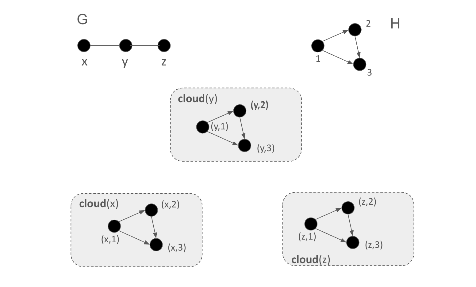
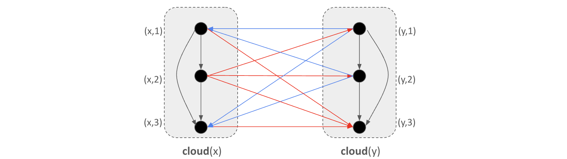
Let $H$ be a digraph and $G$ be an undirected graph (that we call a skeleton). Moreover, we work with a fixed ordering $\sigma:[|V(G)|]\rightarrow V(G)$ of vertices in $G$ , i.e., $(\sigma(1),\sigma(2),\ldots,\sigma(|V(G)|))$ is a permutation of $V(G)$ . The random process $D^{\sigma}_{G}[H]$ generates a product graph $G^{\prime}$ via the following steps: (i) First, start with the vertex set $V(G)$ . Replace each vertex $v\in V(G)$ with a copy $H_{v}$ of digraph $H$ . For each $v$ , we denote by ${\sf cloud}(v)$ the vertex set in the copy $H_{v}$ , that is, ${\sf cloud}(v)=\{(v,a):a\in V(H)\}$ , (ii) Next, for each $\{u,v\}\in E(G)$ , and for all pairs of vertices $a,b\in V(H)$ add either an arc $(u,a)(v,b)$ or $(v,b)(u,a)$ with equal probability (i.e., we pick a random orientation for this pair), and (iii) For each edge $\{u,v\}\not\in E(G)$ such that $u$ appears before $v$ in permutation $\sigma$ and for all pairs of vertices $a,b\in V(H)$ , add arc $(u,a)(v,b)$ . Another way to describe this random process is to first perform an undirected lexicographic product and then orient the $G$ -edges between the clouds at random, while the edges inside the clouds are oriented according to $H$ . See Figure 1 and Figure 2 for illustration of Steps (i) and (ii).

Refer to caption — Figure 1: An illustration of $D^{\sigma}_{G}(H)$ after Step 1. Each vertex of $G$ is replaced by a copy of $H$ .

The following property is easy to see but will be crucial for us.

Observation 7.

The graph $D^{\sigma}_{G}[H]$ is a tournament if and only if $H$ is.

The following lemma is easy to see.

Lemma 8.

Let $H$ be a digraph and $G$ an undirected graph. Then, $\vec{\chi}(D^{\sigma}_{G}[H])\leq\chi(G)\vec{\chi}(H)$ with probability one.

Proof.

Let $X_{1},X_{2},\ldots,X_{g}$ be color classes of $G$ where $g=\chi(G)$ and $Y_{1},\ldots,Y_{h}$ be acyclic color classes of $H$ where $h=\vec{\chi}(H)$ . Since each $X_{i}$ is independent in $G$ and $Y_{j}$ is acyclic in $H$ , we have that $X_{i}\times Y_{j}$ is also acyclic in $D^{\sigma}_{G}[H]$ (regardless of the orientation $\sigma$ ). This gives us $g\cdot h$ acyclic color classes. $\hfill\blacktriangleleft$

Consider a sample $G^{\prime}\sim D^{\sigma}_{G}[H]$ . We say that edge $\{u,v\}\in E(G)$ is $\eta$ -consistent if for every $A_{u}\subseteq{\sf cloud}(u)$ and $A_{v}\subseteq{\sf cloud}(v)$ such that $|A_{u}|,|A_{v}|\geq|V(H)|^{\eta}$ , we have that $G^{\prime}[A_{u}\cup A_{v}]$ contains a cycle. Next, we say that the sample $G^{\prime}\sim D^{\sigma}_{G}[H]$ is $\eta$ -good for $(G,H)$ if every edge $\{u,v\}\in E(G)$ is $\eta$ -consistent.

The following lemma argues that a random product graph is $\eta$ -good with high probability. The proof closely follows [14] (Lemma 4.1).

Lemma 9.

For all $\eta\in(0,1/2]$ , there exists a constant $n_{0}$ (depending on $\eta$ ) such that for all $G$ and $H$ such that $|V(H)|\geq|V(G)|\geq n_{0}$ , the probability that the graph $D^{\sigma}_{G}[H]$ is $\eta$ -good is at least $1-\eta^{2}$ .

Proof.

We need a simple observation: When $G^{\prime}[X]$ is acyclic for subset $X\subseteq V(G^{\prime})$ , some topological ordering $\tau:X\rightarrow[|X|]$ is valid for $X$ (i.e., there is no edge going back in the ordering).

Fix an edge $\{u,v\}\in E(G)$ . We first analyze the probability that $\{u,v\}$ is not $\eta$ -consistent (denote by event ${\mathcal{E}}_{uv}$ ), i.e., there exists $A_{u},A_{v}$ such that $G^{\prime}[A_{u}\cup A_{v}]$ is acyclic. This can be upper bounded by the probability that some topological ordering is valid for $A_{u}\cup A_{v}$ .

$\displaystyle{\mathbb{P}}[{\mathcal{E}}_{uv}]$	$\displaystyle\leq$	$\displaystyle{\mathbb{P}}[(\exists A_{u},A_{v}:\|A_{u}\|,\|A_{v}\|=\|V(H)\|^{\eta})(% \exists\tau)\mbox{ $\tau$ is valid for $A_{u}\cup A_{v}$}]$
	$\displaystyle\leq$	$\displaystyle\|V(H)\|^{2\|V(H)\|^{\eta}}\cdot{\mathbb{P}}[(\exists\tau)\mbox{ $% \tau$ is valid for $A_{u}\cup A_{v}$}]$
	$\displaystyle\leq$	$\displaystyle\|V(H)\|^{2\|V(H)\|^{\eta}}\cdot(2\|V(H)\|^{\eta})!\cdot{\mathbb{P}}[% \tau\mbox{ is valid for $A_{u}\cup A_{v}$}]$

Now consider a fixed $w\in A_{u}\cup A_{v}$ (say $w\in A_{u}$ without loss of generality). Since $w$ is adjacent to all vertices in $A_{v}$ , the ordering $\tau$ necessitates the orientation of all such edges between $w$ and $A_{v}$ . This means that the probability is at most $(1/2)^{|A_{v}|}$ for a fixed $w$ , and therefore

{\mathbb{P}}[\tau\mbox{ is valid for $A_{u}\cup A_{v}$}]\leq(1/2)^{|A_{v}||A_{% u}|}\leq(1/2)^{|V(H)|^{2\eta}}

Plugging this term back, we get:

{\mathbb{P}}[{\mathcal{E}}_{uv}]\leq|V(H)|^{4|V(H)|^{\eta}}\cdot(1/2)^{|V(H)|^% {2\eta}}\leq 2^{-|V(H)|^{2\eta}+4|V(H)|^{\eta}\lg_{2}|V(H)|}

When $|V(H)|$ is sufficiently large, we can make ${\mathbb{P}}[{\mathcal{E}}_{uv}]$ smaller than $\eta^{2}/|V(H)|^{2}$ , and therefore (by the union bound over the edges of $G$ ) the probability that $G^{\prime}$ is not $\eta$ -good is at most $\eta^{2}$ as desired. $\hfill\blacktriangleleft$

2.2.3 New Graph Product Inequality

This subsection presents an analogue of the graph product inequality for our randomized lexicographic product.

Lemma 10 (New inequality).

Let $G$ and $H$ be arbitrary undirected and directed graphs. Let $G^{\prime}\sim D^{\sigma}_{G}[H]$ be such that $G^{\prime}$ is $\eta$ -good for $(G,H)$ . Then, we have that

\vec{\alpha}(G^{\prime})\leq\alpha(G)\cdot\vec{\alpha}(H)+|V(G)||V(H)|^{\eta}.

Proof.

Let $S\subseteq V(G^{\prime})$ be such that $|S|=\vec{\alpha}(G^{\prime})$ and $G^{\prime}[S]$ is acyclic. We partition $S$ into $\bigcup_{v}S_{v}$ where $S_{v}=S\cap{\sf cloud}(v)$ . We say that $S_{v}$ is large if $|S_{v}|\geq|V(H)|^{\eta}$ and small otherwise. Clearly, the total size of the small sets $S_{v}$ is at most $|V(G)|\cdot|V(H)|^{\eta}$ .

Now, for each large set $S_{v}$ , we have that $S_{v}$ induces an acyclic subgraph in $H$ , so $|S_{v}|\leq\vec{\alpha}(H)$ . Define the large clouds $L\subseteq V(G)$ where $L=\{v:S_{v}\mbox{ is large}\}$ . It is clear that $L$ must be an independent set in $G$ : Otherwise, if $u,v\in L$ has an edge $\{u,v\}\in E(G)$ , this would imply that $S_{u}\cup S_{v}$ induces a cycle. Therefore, we have that the total size of large sets is at most $\alpha(G)\cdot\vec{\alpha}(H)$ . $\hfill\blacktriangleleft$

2.2.4 Completing the Proof: The $𝒌$ -Fold Lexicographic Product

Now we complete the proof of Lemma 4. Given undirected graph $\widehat{G}$ and a fixed ordering $\sigma$ of $V(\widehat{G})$ , define a sequence of (random) tournaments $G_{1},\ldots,G_{k}$ as follows:

$\blacksquare$

We construct tournament $G_{1}$ by orienting edges according to the ordering $\sigma$ . That is, $(u,v)\in E(G_{1})$ if and only if $\sigma(u)<\sigma(v)$ . We have that $\vec{\chi}(G_{1}),\vec{\alpha}(G_{1})\leq|V(\widehat{G})|$ .
$\blacksquare$

For all $i\geq 1$ , $G_{i+1}=D^{\sigma}_{\widehat{G}}[G_{i}]$ . Since $G_{1}$ is a tournament, from Observation 7, graph $G_{i}$ must be a tournament for all $i$ .

Our final graph is $T=G_{k}$ . Clearly, we have $|V(G_{i})|=|V(\widehat{G})|^{i}$ and in particular $|V(T)|=|V(\widehat{G})|^{k}$ . The following is a trivial consequence of Lemma 8 (applying it iteratively).

Observation 11.

With probability one, $\vec{\chi}(G)\leq\chi(\widehat{G})^{k-1}|V(\widehat{G})|$ .

Lemma 12.

For sufficiently large $|V(\widehat{G})|$ , the probability that, for all $i\in\{2,\ldots,k\}$ , the graph $G_{i}$ is $(1/k)$ -good for $(\widehat{G},G_{i-1})$ is at least $(1-1/k)$

Proof.

Applying Lemma 9 (notice that the precondition $|V(G_{i})|\geq|V(\widehat{G})|$ is always satisfied), the probability that a fixed $G_{i}$ is not $(1/k)$ -good is at most $1/k^{2}$ . Denote by ${\mathcal{E}}_{i}$ the event that $G_{i}$ is $(1/k)$ -good for $(\widehat{G},G_{i-1})$ .

{\mathbb{P}}[\wedge_{i}{\mathcal{E}}_{i}]=\prod_{i}{\mathbb{P}}[{\mathcal{E}}_% {i}\mid\wedge_{j<i}{\mathcal{E}}_{j}]\geq(1-1/k^{2})^{k}\geq 1-1/k\

$\hfill\blacktriangleleft$

Now assume that all $G_{i}$ are $(1/k)$ -good. From Lemma 10, we have that, for all $i\leq k$ ,

\vec{\alpha}(G_{i})\leq\alpha(\widehat{G})\cdot\vec{\alpha}(G_{i-1})+|V(% \widehat{G})||V(G_{i-1})|^{1/k}\leq\alpha(\widehat{G})\cdot\vec{\alpha}(G_{i-1% })+|V(\widehat{G})|^{2}

It is easy to derive that $\vec{\alpha}(G_{k})\leq O(\alpha(\widehat{G})^{k}|V(\widehat{G})|^{2})$ , thus completing the proof of Lemma 4.

3 Approximation Algorithms

In this section, we provide approximation algorithms to properly color directed graphs promised, directly or indirectly, to have “small” dichromatic number. First, we give an algorithm to color a 2-dicolorable digraph with few colors. Then we extend this to $\ell$ -dicolorable digraphs. Next, we consider digraphs with bounded independence number, a direct generalization of tournaments (which have independence number one). Here, we can obtain bounds when we are given additional promises such as that the input digraph is 2-dicolorable or that it is $C_{3}$ -free. We present some useful observations after presenting some necessary notation.

We define $uv\in A$ to be an arc directed from $u$ to $v$ . For $v\in V$ , let $N^{+}(v)=\{u\nobreak\ |\nobreak\ vu\in A\}$ and $N^{-}(v)=\{u\nobreak\ |\nobreak\ uv\in A\}$ . For $S\subset V$ , we define $N^{+}(S)=\bigcup_{v\in S}N^{+}(v)$ , and we define $N^{-}(S)$ analogously. For $S\subseteq V$ , we use $D[S]$ to denote the digraph induced on the vertex set $S$ , although we frequently abuse notation and refer to the induced subdigraph itself as $S$ . Sometimes, we use $V(D)$ and $A(D)$ to refer to the vertex and arc set, respectively. We use $n$ to denote the number of vertices in $D$ , when it is clear to which digraph $D$ we are referring.

Observation 13.

Let $D$ be a digraph such that $\vec{\chi}(D)\leq\ell$ , for some $1\leq\ell\leq n$ . Then for every (induced) subgraph $D^{\prime}$ of $D$ , there exists a vertex $v\in V(D^{\prime})$ such that $\vec{\chi}(D^{\prime}[N^{+}(v)])\leq\ell-1$ .

Proof.

Since $\vec{\chi}(D)\leq\ell$ , there is a partition of the vertices into $V(D)=\bigcup_{1\leq i\leq\ell}S_{i}$ such that each set $S_{i}$ is acyclic. Now consider an ordering of $V(D)$ which consists of an acyclic ordering of $S_{1}$ (i.e., with no backward arcs from $A(S_{1})$ ) followed by an acyclic ordering of $S_{2}$ , and so on. Notice that the last vertex in this ordering $v$ has $N^{+}(v)\subseteq\bigcup_{1\leq j\leq\ell-1}S_{j}$ , which is $(\ell-1)$ -colorable. $\hfill\blacktriangleleft$

Given a digraph $D$ and a total order $\prec$ on $V(D)$ , let $G_{\prec}$ denote the undirected graph whose edges correspond to arcs of $D$ that are backwards with respect to $\prec$ (i.e., by the arcs $vu\in A(D)$ such that $u\prec v$ ). In other words, we consider all backwards arcs with respect to the ordering $\prec$ and then we ignore the orientation of the arcs, resulting in an undirected backedge graph.

Observation 14 ([26]).

Let $G_{\prec}$ be a backedge graph associated with $D$ and $\prec$ . Then $\vec{\chi}(D)\leq\chi(G_{\prec})$ . Moreover, any proper coloring of vertices of $G_{\prec}$ is also a proper coloring for $D$ .

This follows from the fact that every stable set in $G_{\prec}$ is acyclic in $D$ . Recall that $d$ -degenerate (undirected) graph is one in which there is a vertex ordering such that each vertex has at most $d$ neighbors to the left.

Observation 15 (Folklore).

A $d$ -degenerate graph is $(d+1)$ -colorable and such a coloring can be computed in polynomial time.

A digraph $D$ is $d$ -out-degenerate if every induced subgraph of $D$ contains a vertex with out-degree at most $d$ . An implication of Observation 14 and 15 is the following.

Observation 16.

A $d$ -out-degenerate digraph is $(d+1)$ -colorable and such a coloring can be computed in polynomial time.

We remark that we will always assume that a digraph $D$ that we want to color is strongly connected; if this were not the case, we can color each strongly connected component separately, using the same color palette.

3.1 Coloring $\ell$ -Dicolorable Digraphs

We now consider the case in which we are promised an upper bound on the dichromatic number of an input digraph and the goal is to color it with few colors. We first consider the case in which the input digraph $D$ is promised to be 2-colorable. Recall that coloring such a digraph with two colors, even when it is oriented, is $\mathsf{NP}$ -hard [5]. We present Algorithm 1 and use it to prove Theorem 17.

Theorem 17.

Given a digraph $D$ with $\vec{\chi}(D)\leq 2$ , there exists a polynomial-time algorithm to properly color $D$ with at most $2\sqrt{n}$ colors.

Algorithm 1 has a similarity to Wigderson’s algorithm for coloring 3-colorable graphs [27]. However, one key difference between coloring 3-colorable graphs and coloring 2-dicolorable digraphs is that in the case of the former, each vertex has a neighborhood that is easy to color, since each vertex neighborhood is bipartite. In the latter case, we are only guaranteed the existence of two vertices, whose out-neighborhoods are acyclic and are therefore easy to color, and both of these vertices might have small out-degree, preventing us from making progress. We circumvent this issue by finding another way to remove small-degree vertices, using Observation 14.

Algorithm 1 Dicoloring(

D

).

Proof of Theorem 17.

We use the following claims to prove the correctness of Algorithm 1.

Claim 18.

In Step 2 of Algorithm 1, we assign at most $\sqrt{n}$ colors from colors $\{1,\ldots,\sqrt{n}\}$ .

Proof.

Since each time we use a new color we remove at least $\sqrt{n}$ vertices, we assign at most $\sqrt{n}$ colors in Step 2. $\hfill\vartriangleleft$

Claim 19.

The coloring assigned by Algorithm 1 is a proper coloring.

Proof.

First, observe that the backedge graph $G_{\prec}$ corresponding to $D[S]$ and $\prec$ is ( $\sqrt{n}-1$ )-degenerate. Hence we can properly color $G$ using $\sqrt{n}$ colors from $\{\sqrt{n},\ldots,2\sqrt{n}\}$ ²²2Notice that if we actually assign $\sqrt{n}$ colors in Step 2, then we have colored the whole graph. So if we reach Step 4, we can begin with color $\sqrt{n}$ . due to Observation 15. Moreover, due to Observation 14, this coloring is a proper coloring for $D[S]$ . Finally, since we assign a unique color from $\{1,\ldots,\sqrt{n}\}$ (distinct from colors assigned to vertices of $D[S]$ ) to an acyclic subdigraph of $D$ in each iteration of Step 2, this directly extends to a proper coloring of $D$ . $\hfill\vartriangleleft$

Since we assign at most $\sqrt{n}$ colors in Step 2 and at most $\sqrt{n}$ colors in Step 3–5 (Observation 15), we use a total of at most $2\sqrt{n}$ many colors to color $D$ . $\hfill\blacktriangleleft$

We remark that Algorithm 1 can easily be modified so that, on an input digraph $D$ that is not 2-dicolorable, it either outputs a coloring of $D$ with at most $2\sqrt{n}$ colors or outputs an induced subgraph of $D$ in which no vertex has an acyclic out-neighborhood, which is a proof that $D$ is not 2-dicolorable.

A positive answer to the following question would immediately yield an improved bound on the number of colors needed to color a 2-colorable digraph.

Question 1.

Given a 2-dicolorable $d$ -out-degenerate digraph $D$ , can we find a coloring of $D$ using at most $d^{1-\epsilon}$ colors in polynomial time?

Next, we provide a $O(n^{2\ell})$ -time algorithm to color a digraph $D$ with $\vec{\chi}(D)\leq\ell$ using at most $O(n^{1-\frac{1}{\ell}})$ colors, which we use to prove Theorem 20, of which Theorem 17 is a special case.

Algorithm 2 DicoloringGeneral(

D

,

\ell+1

).

Theorem 20.

Given a digraph $D$ with $\vec{\chi}(D)\leq\ell$ , there exists an algorithm to properly color $D$ with at most $\ell\cdot n^{1-\frac{1}{\ell}}$ colors in time $O(n^{2\ell})$ .

Proof.

We will prove Theorem 20 using Algorithm 2. Let $D$ be a digraph such that $\vec{\chi}(D)\leq\ell+1$ . Due to Observation 13, there exists at least one vertex $v\in V(D)$ such that $\vec{\chi}(N^{+}(v))\leq\ell$ . Thus, each time we run Step 2, Step (b) will find a successful vertex. Let us assume by induction that DicoloringGeneral( $D^{\prime}$ , $\ell$ ) returns a coloring of $D^{\prime}$ using at most $\ell\cdot V(D^{\prime})^{1-\frac{1}{\ell}}$ colors in $O(V(D^{\prime})^{2\ell})$ time when $\vec{\chi}(D^{\prime})\leq\ell$ . Notice that this statement is true in the base case when $\ell=2$ by Theorem 17. We use the following claim.

Claim 21.

The maximum value of $i$ in an execution of Algorithm 2 is at most $\ell\cdot n^{1-\frac{1}{\ell+1}}$ .

Proof.

Observe that the value of $i$ increases only in Step 2(d) of Algorithm 2, and this occurs when we color some (at least $n^{1-\frac{1}{\ell+1}}$ ) vertices of $D$ . Suppose this process occurs $q$ times; that is, there are $q$ disjoint sets of vertices $S_{1},\ldots,S_{q}$ such that $S_{j}$ is colored in the $j$ ’th execution of Step 2(b) of Algorithm 2 using at most $\ell\cdot|S_{j}|^{1-\frac{1}{\ell}}=\ell\cdot|S_{j}|^{\frac{\ell-1}{\ell}}$ colors. Then we have

\displaystyle q\cdot n^{1-\frac{1}{\ell+1}}\leq_{j\in[q]}|S_{j}|\leq n\quad% \Rightarrow\quad q\leq n^{\frac{1}{\ell+1}}.

At the end of the algorithm, $i=\sum_{j\in[q]}\ell\cdot|S_{j}|^{\frac{\ell-1}{\ell}}$ . To complete the proof, we need to establish that $\sum_{j\in[q]}\ell\cdot|S_{j}|^{\frac{\ell-1}{\ell}}\leq\ell\cdot n^{1-\frac{1% }{\ell+1}}$ . Letting $n_{j}=|S_{j}|$ and noting that the function $f(x)=x^{\frac{\ell-1}{\ell}}$ is concave, we have by Jensen’s inequality,
$\displaystyle\sum_{j\in[q]}n_{j}^{\left(\frac{\ell-1}{\ell}\right)}\leq q\bigg% (\frac{1}{q}\sum_{j\in[q]}n_{j}\bigg)^{\frac{\ell-1}{\ell}}\leq q\left(\frac{n% }{q}\right)^{\frac{\ell-1}{\ell}}=q^{\frac{1}{\ell}}n^{\frac{\ell-1}{\ell}}% \leq(n^{\frac{1}{\ell+1}})^{\frac{1}{\ell}}n^{\frac{\ell-1}{\ell}}=n^{\frac{% \ell}{\ell+1}}=n^{1-\frac{1}{\ell+1}}.$

This completes the proof of the claim. $\hfill\vartriangleleft$

Thus, due to Claim 21, we have that the total number of colors used in Step 2 of Algorithm 2 is at most $\ell\cdot n^{1-\frac{1}{\ell+1}}$ . Since we use at most $n^{1-\frac{1}{\ell+1}}$ colors in Step 4 and 5 of the algorithm, we have that the total number of colors used by Algorithm 2 is at most $(\ell+1)\cdot n^{1-\frac{1}{\ell+1}}$ . Finally, the running time follows from the fact that after at most $n$ invocations of the subroutine to color $\ell$ -colorable digraphs using at most $\ell\cdot n^{1-\frac{1}{\ell}}$ colors, we remove the (non-empty) out-neighborhood of at least one vertex from the digraph $D$ . Thus, we call the subroutine DicolorGeneral( $D^{\prime}$ , $\ell$ ) at most $n^{2}$ times for a total running time of $O(n^{2}n^{2\ell})=O(n^{2(\ell+1)})$ . $\hfill\blacktriangleleft$

3.2 Coloring Digraphs with Bounded Independence Number

We now consider digraphs which have bounded independence number. The independence number of a digraph is the size of the maximum independent set of its underlying undirected graph. Tournaments are a well-studied class of digraphs with independence number one. Digraphs with bounded independence number are sometimes referred to as dense digraphs, since for fixed independence number $\alpha$ , they have a quadratic number of edges.

One can hope that some of the algorithmic results for tournaments can be extended to general digraphs parametrized by independence number. In this section, we show that this is the case (i) when we consider digraphs promised to be 2-dicolorable, and (ii) when we consider oriented digraphs with no $C_{3}$ , where $C_{k}$ is a cyclically oriented cycle on $k$ vertices. The latter result improves upon a bound given by [18] via a simpler algorithm.

We refer to the set of vertices that have no arc from or towards $v$ as its non-neighborhood $N^{o}(v)$ (i.e., $N^{o}(v)=V\setminus\{N^{+}(v)\cup N^{-}(v)\cup v\}$ ). We say there is a non-edge between $u$ and $v$ if there is no arc in $A$ from $u$ to $v$ or from $v$ to $u$ . If we are referring to an non-edge with a fixed direction (i.e., a non-edge $e=uv$ ), then we refer to it as a non-arc. Notice that if $u v$ is a non-arc, then there is a non-edge between $u$ and $v$ (i.e., if $u v$ is an arc, then we do not say that $v u$ is a non-arc). For an arc or non-arc $e=uv$ , we use $N(e)$ to denote the vertices in $N^{+}(v)\cap N^{-}(u)$ .

The following observation is useful in digraphs with bounded independence number.

Observation 22.

Let $D$ be a digraph with independence number at most $\alpha$ . Then for every vertex $v\in V(D)$ , the digraph $D[N^{o}(v)]$ has independence number at most $\alpha-1$ .

One of the main tools presented in [21] for coloring tournaments is a path decomposition, in which a tournament is decomposed into vertex sets, which are essentially the neighborhoods of arcs on a shortest path between two vertices $s$ and $t$ , where $N(e)$ (defined above) is the neighborhood of arc $e$ . Moreover, if $s$ and $t$ are chosen such that $N^{+}(s)$ and $N^{-}(t)$ each have small dichromatic number and $N(e)$ has small dichromatic number for each arc $e$ on the shortest path, then this decomposition can be used to show that the whole tournament has small dichromatic number. The main idea is that we can reuse color palettes for neighborhoods of arcs that are far apart on the shortest path, because arcs between these neighborhoods must go backwards, otherwise it would contradict the minimality of the shortest path.

In this section, we adapt this path decomposition to oriented digraphs by taking a shortest path – not just of arcs – but of arcs and non-arcs (in other words, non-edges can be included in the shortest path to be traversed in either direction). Thus, we can fix some pair of vertices $s$ and $t$ , and then we can partition the vertex set of a digraph into neighborhoods of arcs on the shortest path and non-neighborhoods of vertices on the shortest path. We can still ensure that arcs between neighborhoods of arcs and arcs between non-neighborhoods of vertices that are far apart on the shortest path must go backwards, allowing us to reuse a relatively small color palette to color all the vertices of the digraph, except $N^{+}(s)$ and $N^{-}(t)$ , which must therefore be chosen carefully.

Hence, to apply the path decomposition, the main challenges are finding a good vertex pair $s, t$ such that $N^{+}(s)$ and $N^{-}(t)$ each have small dichromatic number, and showing that the non-neighborhoods of the vertices and the neighborhoods of the arcs or non-arcs on a shortest path from $s$ to $t$ each have small dichromatic number. However, we can define the decomposition for any $s, t$ vertex pair.

3.2.1 Decomposition for Digraphs

In this section, we define a decomposition for digraphs based on a shortest path from $s$ to $t$ for any vertex pair $s$ and $t$ . In the next definition, we have $v_{0}:=s$ and $v_{k}:=t$ .

Definition 23.

We define a vertex chain $(v_{i})_{0\leq i\leq k}$ of a digraph $D$ as follows: Let $v_{0}$ and $v_{k}$ be a pair of vertices and let $(v_{i})_{0\leq i\leq k}$ be the vertices in the shortest path from $v_{0}$ to $v_{k}$ , where the path may consist of both forward arcs and non-arcs (but no backward arcs). If in addition, $\vec{\chi}(N^{+}(v_{0}))\leq b$ and $\vec{\chi}(N^{-}(v_{k}))\leq b$ , then we call it a $b$ -vertex chain.

We remark that in the above definition, $v_{0}$ and $v_{k}$ are not necessarily distinct, in which case the vertex chain consists of a single vertex and the shortest path has length zero.

Additionally, we define an edge chain $(e_{i})_{1\leq i\leq k}$ corresponding to a vertex chain, where $e_{i}$ is the arc or non-arc from $v_{i-1}$ to $v_{i}$ . We build zones that can be efficiently colored, and such that arcs between zones at distance more than four (i.e., long arcs) go backwards.

Definition 24.

Given a vertex chain $(v_{i})_{0\leq i\leq k}$ , a path decomposition of a digraph $D$ is defined as:

$\blacksquare$

$D_{1}=N(e_{1})$ .
$\blacksquare$

For $2\leq i\leq k$ , $D_{i}=N(e_{i})\setminus(\cup_{1\leq j\leq i-1}D_{j})$ .
$\blacksquare$

For $0\leq i\leq k$ , $N_{i}=N^{o}(v_{i})\setminus{(\cup_{1\leq j\leq k}D_{j}\cup_{0\leq j\leq i-1}N_% {j})}$ .
$\blacksquare$

$D_{0}=N^{+}(v_{0})\setminus(\cup_{1\leq j\leq k}(D_{j}\cup N_{j})\cup N_{0})$ .
$\blacksquare$

$D_{k+1}=N^{-}(v_{k})\setminus\cup_{0\leq j\leq k}(D_{j}\cup N_{j})$ .
$\blacksquare$

$Z=V\setminus(\cup_{0\leq j\leq k}(D_{j}\cup N_{j})\cup D_{k+1})$ .

First we prove that this is indeed a decomposition of $D$ .

Lemma 25.

Let $D=(V,A)$ be a digraph, and $(D_{0},\ldots,D_{k+1},N_{0},\ldots,N_{k},Z)$ be a path decomposition of $D$ . Then $Z\subseteq\{v_{0},v_{k}\}$ .

Proof.

We will prove this by contradiction. Suppose there is a vertex $w\in V\setminus\{v_{i}\}_{0\leq i\leq k}$ that does not belong to any $D_{i}$ or $N_{i}$ . Since $w$ does not belong to $D_{0}$ or to $D_{k+1}$ (nor to $N_{0}$ or $N_{k}$ ), then $w\in N^{-}(v_{0})$ and $w\in N^{+}(v_{k})$ . Take the smallest integer $i$ such that $w\in N^{+}(v_{i})$ . There must be one since $w\in N^{+}(v_{k})$ . Notice that $i\geq 1$ since $w\in N^{-}(v_{0})$ . Since $w\notin N^{o}(v_{i-1})$ , then $w\in N(e_{i})$ . Therefore, $w\in D_{i}$ , which is a contradiction.

We note that each vertex in the vertex chain $(v_{i})_{0\leq i\leq k}$ belongs to a $D_{i}$ or $N_{i}$ , except in the case where $k=0$ or $k=1$ . In this case, we add this set of at most two remaining vertices to $Z$ . Finally, we remark that the decomposition is actually a partition of $V$ . $\hfill\blacktriangleleft$

We now show that long arcs between $N_{i}$ ’s or between $D_{i}$ ’s go backwards. Since the $N_{i}$ s and $D_{i}$ s will be colored with different color palettes, we do not need to worry about arcs between an $N_{i}$ and a $D_{j}$ .

Lemma 26.

Let $0\leq i,j\leq k+1$ such that $j\geq i+5$ . For $u\in D_{i}$ and $w\in D_{j}$ , we have $u\in N^{+}(w)$ . Furthermore, if $u\in N_{i}$ and $w\in N_{j-1}$ , we have $u\in N^{+}(w)$ .

Proof.

We will prove this by contradiction. Suppose $j\geq i+5$ and $u\in N^{-}(w)$ (respectively, $u\in N^{o}(w)$ ). Then there is a path of three arcs (respectively, of two arcs and one non-arc) from $v_{i}$ to $v_{j-1}$ , namely $(v_{i},u,w,v_{j-1})$ . (By definition of the decomposition, $u\in D_{i}$ implies $u\in N^{+}(v_{i})$ and $w\in D_{j}$ implies $w\in N^{-}(v_{j-1})$ .) This is not possible since by the definition of the vertex chain as the shortest path, there can be no path between $v_{i}$ and $v_{j-1}$ with fewer than four arcs (since $(j-1)-i\geq(i+5-1)-i=4$ ). Finally, if $u\nobreakspace\in N_{i}$ and $w\in N_{j-1}$ , $(v_{i},u,w,v_{j-1})$ is also a path (of forward arcs and non-arcs) of length three from $v_{i}$ to $v_{j-1}$ , which as previously is a contradiction. $\hfill\blacktriangleleft$

The following lemma demonstrates how the vertex chain and path decomposition can be used to color digraphs.

Lemma 27.

If $D$ has a $b$ -vertex chain that can be found in polynomial time and if $\vec{\chi}(N(e))\leq c$ for each arc and non-arc $e$ , and $\vec{\chi}(N^{o}(v))\leq d$ for every vertex $v$ , then

\vec{\chi}(D)\leq\begin{cases}5c+4d+2(b-c)&\text{if }b>c,\\ 5c+4d&\text{if }b\leq c.\end{cases}

Furthermore, if there are no arcs from $D_{0}$ to $D_{k+1}$ and $\max\{b,c,d\}=b$ , then $\vec{\chi}(D)\leq 4c+4d+b$ .

Proof.

Given a $b$ -vertex chain, we construct a path decomposition as per Definition 23. We make five palettes of $c$ colors each with labels from $0$ to $4$ . We color each $D_{i}$ using the color palette with label $i\bmod 5$ . Note that the sets $D_{0}$ and $D_{k+1}$ each require $b-c$ extra colors in their palettes if $b>c$ .

Next, we make four different palettes of $d$ colors each with labels from $5$ to $8$ . We color each $N_{i}$ using the color palette with label $5+(i\bmod 4)$ . The set of colors used is of size $d$ for every $N_{i}$ , thus we can efficiently color each set by the assumption of the lemma.

Our goal is now to prove that this is a proper coloring of the digraph $D$ . We will do this by showing that all forward arcs between different $D_{i}$ or $N_{i}$ are bicolored. By Lemma 26, there are no forward arcs between $D_{i}$ and $D_{j}$ when $j\geq i+5$ , or $N_{i}$ and $N_{j}$ with $j\geq i+4$ . Furthermore, by the definition of the coloring, no vertex in $D_{i}$ and $D_{j}$ can share a color for $i+1\leq j\leq i+4$ , and the same goes for vertices in $N_{i}$ and $N_{j}$ with $i+1\leq j\leq i+3$ . Thus all forward arcs from $D_{i}$ to $D_{j}$ or $N_{i}$ to $N_{j}$ will be bicolored. Since every $D_{i}$ and $N_{i}$ is properly colored, and all forward arcs between different $D_{i}$ are bicolored, the unions of $D_{i}$ ’s and the union of $N_{i}$ ’s are both properly colored. Since these two sets use disjoint color palettes, and because every vertex is in some $D_{i}$ or $N_{i}$ (by Lemma 25), the whole digraph $D$ is properly colored. Furthermore, we note that if there are no arcs from $D_{0}$ to $D_{k+1}$ , then we can save $b-c$ colors resulting in the claimed bound.

Finally, we remark that if the vertex chain consists of at most two vertices, then we have $\vec{\chi}(D)\leq 2d+c+2b+2$ , since we can decompose $D$ into (possibly some subset of) $Z,N_{0},N_{1},D_{0},D_{k}$ and $D_{k+1}$ . In the case where there are no arcs from $D_{0}$ to $D_{k+1}$ , we have $\vec{\chi}(D)\leq 2d+c+2+b$ . $\hfill\blacktriangleleft$

3.2.2 Coloring 2-Dicolorable Dense Digraphs

In this section, our goal is to prove Theorem 28.

Theorem 28.

Let $D$ be a 2-dicolorable digraph with independence number $\alpha$ . Then a coloring with at most $\frac{10}{3}(4^{\alpha}-1)$ colors can be found in polynomial time.

We say an arc $e$ in $D$ is heavy if $N(e)$ contains a directed cycle. Moreover, we say a non-edge between $u$ and $v$ is heavy if $N^{+}(u)\cap N^{-}(v)$ or if $N^{+}(v)\cap N^{-}(u)$ contains a directed cycle. If a digraph contains no heavy arcs and no heavy non-edges, then it is light. In the case of 2-colorable tournaments, we can partition the vertex set into two tournaments such that no arc is heavy [21], but in the case of 2-colorable digraphs we still need to account for the non-arcs. To do this, we will add a step before this partition.

Lemma 29.

A 2-colorable digraph $D$ can be transformed into a 2-colorable digraph $D^{\prime}$ with no heavy non-arc by adding arcs.

Proof.

Let $e$ be a heavy non-arc between $u$ and $v$ . Without loss of generality, suppose that there is a directed cycle in $N^{+}(u)\cap N^{-}(v)$ . This cycle must be colored with two colors, thus $u$ , $v$ and any $z\in N^{-}(u)\cap N^{+}(v)$ cannot all be colored the same color, else there would be a monochromatic 4-cycle. Therefore, we can add the arc from $u$ to $v$ , since it will not lead to any monochromatic cycle in a 2-coloring of $D$ . So we can construct $D^{\prime}$ by starting from $D$ , and while there are still heavy non-arcs, we add an arc between two vertices in the way we just described. $\hfill\blacktriangleleft$

After applying Lemma 29, we obtain a digraph in which every non-arc is light. (Of course, we have not increased the independence number, since we have not removed any arcs.) If a digraph contains a digon (i.e., a directed 2-cycle), then both arcs can be considered to be heavy, since the endpoints must have different colors. Since the endpoints of heavy arcs must have different colors, they cannot contain any odd cycles in a 2-coloring. In other words, the set of heavy arcs forms a bipartite graph and we can therefore partition the set of vertices in order to cut all heavy arcs. This results in the following corollary.

Corollary 30.

Let $D$ be a 2-colorable digraph. Then $D$ can be partitioned into two light oriented 2-colorable digraphs $D_{1}$ and $D_{2}$ such that $\vec{\chi}(D)\leq\vec{\chi}(D_{1})+\vec{\chi}(D_{2})$ .

Since finding this partition is equivalent to finding a bipartition of a bipartite graph, it can be found in polynomial time. Next, we prove another useful observation.

Observation 31.

Let $D$ be a $k$ -colorable digraph. Then there exist vertices $u$ and $w$ such that $D[N^{+}(u)\cup N^{-}(w)]$ is $(k-1)$ -colorable.

Proof.

Since $D=(V,A)$ is $k$ -colorable, there exist $k$ transitive sets $X_{1},\ldots,X_{k}$ such that $V=\cup_{i=1}^{k}X_{i}$ . Then take $u$ to be the vertex in $X_{1}$ that has only incoming arcs (or non-arcs) from other vertices in $X_{1}$ (i.e., the sink vertex for $X_{1}$ ). Similarly, take $w$ to be the vertex in $X_{1}$ that has only outgoing arcs (or non-arcs) to other vertices in $X_{1}$ (i.e., the source vertex for $X_{1}$ ). The out-neighborhood of $u$ and the in-neighborhood of $w$ are both subsets of $V\setminus{X_{1}}$ , and thus so is their union, which is therefore $(k-1)$ -colorable. $\hfill\blacktriangleleft$

Now we are ready to prove Theorem 28. We use a subroutine for coloring a light, 2-colorable digraph whose steps are shown in Algorithm 3.

Algorithm 3 DicoloringLightIND(

D,\alpha,P

).

Proof of Theorem 28.

We begin by using Lemma 29 to transform the input digraph $D$ into a digraph containing no heavy non-arcs. Next, if $D$ is not a light digraph, we partition $D$ into two light $2$ -colorable digraphs $D_{1},D_{2}$ using Corollary 30.

Then we color light digraphs $D_{1}$ and $D_{2}$ separately using different color palettes. To color, say, $D_{1}$ , we use a recursive algorithm, whose steps are shown in Algorithm 3. (Notice that this presentation includes some technical implementation details on how to distribute the color palettes during the recursive steps.) First, we find a $1$ -vertex-chain in $D_{1}$ . To do this, we apply Observation 31, which takes at most $O(n^{2})$ time (where $n=|V(D_{1})|$ ), by guessing all pairs of endpoints $s, t$ , and checking if the subgraph $D_{1}[N^{+}(s)\cup N^{-}(t)]$ is acyclic. Once we have $s$ and $t$ , we find a 1-vertex chain $(v_{i})_{0\leq i\leq k}$ where $v_{0}=s$ and $v_{k}=t$ . Since $D_{1}$ is light, we have $\vec{\chi}(e_{i})\leq 1$ for each arc and each non-arc $e_{i}$ (since each non-arc is light) in the corresponding edge-chain. Moreover, the independence number of each $N_{i}$ is at most $\alpha-1$ by Observation 22.

In order to prove the upper bound on the number of colors stated in the theorem, we define $f(\alpha)$ to be a function such that $f(\alpha)\geq\vec{\chi}(D)$ for every 2-colorable digraph $D$ with independence number $\alpha$ . Our goal is to find an upper bound on $f(\alpha)$ . Additionally, we define $f_{l}(\alpha)$ to be a function such that $f_{l}(\alpha)\geq\vec{\chi}(D)$ for every 2-colorable light digraph. By Corollary, 30 we have $f(\alpha)\leq 2\cdot f_{l}(\alpha)$ . By Lemma 27, we have the following claim.

Claim 32.

$f_{l}(\alpha)=5+4\cdot f_{l}(\alpha-1)$ .

The base case is $f_{l}(1)=5$ , by [21]. A simple calculation leads to the upper bound in the statement of Theorem 28.

It remains to show that Algorithm 3 runs in polynomial time in $n$ (the size of $V(D_{1})$ ). As noted above, we can find a 1-vertex chain and a corresponding path decomposition in polynomial time. Thus, we partition $V(D_{1})$ into $D_{i}$ ’s and $N_{i}$ ’s, where each $D_{1}[N_{i}]$ has independence number at most $\alpha-1$ . We color each $D_{i}$ in polynomial time and recurse on the $N_{i}$ s. Since no vertex is considered in more than one recursive call for a given $\alpha$ , this leads to at most $\alpha n\leq n^{2}$ recursive calls, resulting in a polynomial-time termination of Algorithm 3. $\hfill\blacktriangleleft$

3.2.3 Coloring $C_{3}$ -Free Dense Digraphs

In this section, $D=(V,A)$ is a $C_{3}$ -free oriented graph with independence number $\alpha(D)$ . Recall that $C_{k}$ denotes a cyclicly oriented $k$ -cycle. Since adding arcs does not decrease the dichromatic number or increase the independence number, we can assume that $D$ is maximally triangle-free, which means that for any pair of vertices $u, v$ in $V$ with no arc between them, both arcs $u v$ and $v u$ would each create a $C_{3}$ in $D$ . In other words, if there is no arc between $u$ and $v$ , then there is a $C_{4}$ in $D$ containing $u$ and $v$ . We will call such a digraph a maximally $C_{3}$ -free digraph. We denote the total out-neighborhood (respectively, in-neighborhood) of a vertex subset $S$ by $N^{+}_{t}(S)$ (respectively, $N^{-}_{t}(S)$ ). A vertex $w\notin S$ belongs to $N^{+}_{t}(S)$ if for all $s\in S$ , we have arc $sw\in A$ . The goal of this section is to prove the following theorem.

Theorem 33.

Let $D$ be a $C_{3}$ -free digraph with independence number $\alpha$ . Then $D$ can be colored with at most $\frac{(\alpha+8)!}{9!}$ colors in polynomial time.

This improves on the previous bound of $\vec{\chi}(D)\leq 35^{\alpha-1}\alpha!$ proved by [18]. Notice that if $D$ is a $C_{3}$ -free digraph and $\alpha(D)=1$ , then $D$ is acyclic (i.e., $\vec{\chi}(D)=1$ ). To prove this result, we will again use the path decomposition presented in Definition 23. When $D$ is a $C_{3}$ -free digraph, this decomposition has additional useful properties.

Observation 34.

Let $D$ be a $C_{3}$ -free digraph. For a vertex chain $(v_{i})_{0\leq i\leq k}$ and a corresponding path decomposition in $D$ , there is no arc from $D_{0}$ to $D_{k+1}$ .

Proof.

Consider a vertex $v\in D_{k+1}$ . Since $v\notin N_{0}$ and $v\notin D_{0}$ , it follows that $v\in N^{-}(v_{0})$ . Thus, for some $u\in D_{0}$ , if there is an arc $u v$ , then there is a $C_{3}$ in $D$ , a contradiction. $\hfill\blacktriangleleft$

By Lemma 27, Observation 34 allows us to color $D_{0}$ and $D_{k+1}$ with the same color palette. This is useful when $D_{0}$ and $D_{k+1}$ require many more colors than $N(e_{i})$ . Let $g(\alpha)$ denote the maximum dichromatic number of a $C_{3}$ -free digraph with independence number at most $\alpha$ .

Lemma 35.

Let $D$ be a maximally $C_{3}$ -free digraph. If $u v$ is a non-arc in $D$ , then $\vec{\chi}(N(uv))\leq g(\alpha-1)$ .

Proof.

Let $a$ be a vertex in $N(uv)$ . Since $u v$ is a non-arc, there is also no edge between $u$ and $v$ . Thus, it must be the case that adding arc $v u$ causes a $C_{3}$ , say with $w$ . So then $N(uv)\subseteq N^{o}(w)$ . If this were not the case, then we would have either triangle $w v a$ or $w a u$ , which is a contradiction. $\hfill\blacktriangleleft$

Lemma 36.

Let $D$ be a maximally $C_{3}$ -free digraph with independence number at most $\alpha$ . $D$ has vertices $s_{1},s_{2}\in V$ such that $\vec{\chi}(N^{-}(s_{1}))\leq\alpha\cdot g(\alpha-1)$ and $\vec{\chi}(N^{+}(s_{2}))\leq\alpha\cdot g(\alpha-1)$ .

Proof.

Find a semi-kernel $K$ in $D$ . A semi-kernel is an independant and distance-2 dominating set in a digraph and can be found in polynomial time [6]. First, we claim that $N^{-}_{t}(K)$ is empty. If not, then there is a vertex $y\in N^{-}_{t}(K)$ , and $y$ is not dominated by any vertex in $K$ (since our digraph does not contain digons). Thus there exists a vertex $v\in K$ such that $v$ 2-dominates $y$ , while $y v$ is an arc by definition of $N^{-}_{t}(K)$ which gives a $C_{3}$ in $D$ , a contradiction.

Now denote by $U$ the set of vertices not in any non-neighborhood $N^{o}(v)$ of a vertex $v\in K$ . In other words, a vertex $u$ is in $U$ if $u$ has an arc to or from each vertex in $K$ . For each vertex $u\in U$ , define $N_{u}=N^{-}(u)\cap K$ , which gives a subset family of size $|U|$ on $K$ . Among them pick a minimal one, say $N_{u^{\prime}}$ , and then arbitrarily choose a vertex $s_{1}\in N_{u^{\prime}}$ . We claim that $\vec{\chi}(N^{-}(s_{1}))\leq\alpha\cdot g(\alpha-1)$ .

For any in-neighbor $w$ of $s_{1}$ , either $w$ lies in non-neighborhood of some vertex in $K-s_{1}$ , or $w\in U$ . The former case can be covered by $(\alpha-1)g(\alpha-1)$ colors since $|K|\leq\alpha$ . Next we prove that in the latter case, $w\in N^{o}(u^{\prime})$ . Note that $ws_{1}$ and $s_{1}u^{\prime}$ are arcs by definition. As in the proof of Lemma 35, it suffices to find $v^{\prime}$ such that $v^{\prime}w$ and $u^{\prime}v^{\prime}$ are arcs. We claim that there must exist such a $v^{\prime}\in K$ . Suppose not, then $N_{w}\subsetneq N_{u^{\prime}}$ , contradicting the fact that $N_{u^{\prime}}$ is minimal since $w,u^{\prime}\in U$ and $s_{1}\in N_{u^{\prime}}$ but $s_{1}\notin N_{w}$ . Thus $\vec{\chi}(N^{-}(s_{1}))\leq(\alpha-1)g(\alpha-1)+g(\alpha-1)=\alpha\cdot g(% \alpha-1)$ .

By reversing the direction of all arcs, the same argument results in a vertex $s_{2}$ such that $\vec{\chi}(N^{+}(s_{2}))\leq\alpha\cdot g(\alpha-1)$ . (Note that $s_{1}$ and $s_{2}$ need not be distinct.) $\hfill\blacktriangleleft$

The following corollary of Lemma 36 that shall be useful in simplifying the presentation of Algorithm 4.

Corollary 37.

Let $D$ be a maximally $C_{3}$ -free digraph with independence number at most $\alpha$ . Then, in polynomial time, we can find vertices $s, t$ such that each $N^{+}(s)$ and $N^{-}(t)$ can be partitioned into at most $\alpha$ components $S_{1},\ldots,S_{\alpha}$ and $T_{1},\ldots,T_{\alpha}$ , respectively, such that for $1\leq j\leq\alpha$ , $D[S_{j}]$ and $D[T_{j}]$ each has independence number at most $\alpha-1$ .

We are now ready to prove Theorem 33 via the algorithm whose steps are detailed in Algorithm 4.

Proof of Theorem 33.

We give an overview of Algorithm 4. Consider a maximally $C_{3}$ -free digraph $D$ with independence number $\alpha$ . By Lemma 36, we can find a pair of vertices $s, t$ such that $\vec{\chi}(N^{+}(s))\leq\alpha\cdot g(\alpha-1)$ and $\vec{\chi}(N^{-}(t))\leq\alpha\cdot g(\alpha-1)$ . Next, we find a $b$ -vertex chain $(v_{i})_{0\leq i\leq k}$ , where $v_{0}=s,v_{k}=t$ and $b=\alpha\cdot g(\alpha-1)$ . For every non-arc $e_{i}$ in the corresponding edge-chain, we have $\vec{\chi}(N(e_{i}))\leq g(\alpha-1)$ due to Lemma 35. For every arc $e_{i}$ , observe that $N(e_{i})$ is empty, since $D$ is $C_{3}$ -free. Thus, for each $D_{i}$ for $1\leq i\leq k$ in the path decomposition, we have $\vec{\chi}(D_{i})\leq g(\alpha-1)$ . Additionally, each $D[N_{i}]$ has independence number at most $\alpha-1$ by Observation 22 and thus has $\vec{\chi}(N_{i})\leq g(\alpha-1)$ . Applying Lemma 27 and Observation 34, implies the following claim.

Claim 38.

$g(\alpha)\leq(\alpha+8)g(\alpha-1)$ .

The base case is $g(1)=1$ , since a $C_{3}$ -free tournament is acyclic. A simple calculation leads to the upper bound stated in the theorem. It remains to show that Algorithm 4 runs in polynomial time. Since an execution of the algorithm on $D$ makes at most $\alpha+8$ recursive calls on subdigraphs with independence number $\alpha-1$ , and these respective subdigraphs are vertex disjoint, each vertex is included in at most $\alpha n\leq n^{2}$ recursive calls, resulting in a polynomial-time termination. $\hfill\blacktriangleleft$

Algorithm 4 Dicoloring

C_{3}

-Free(

D,\alpha,P

).

We conclude this section with the following conjecture.

Conjecture 39.

In an oriented $C_{3}$ -free digraph $D$ with independence number $\alpha$ , there is a vertex $v$ such that $D[N^{+}(v)]$ has independence number $\alpha-1$ .

A proof of this conjecture would imply a singly exponential bound on the dichromatic number for $C_{3}$ -free digraphs (i.e., of the form $c^{\alpha}$ ). Specifically, in Claim 38, we would have $g(\alpha)\leq 9\cdot g(\alpha-1)$ . Conjecture 39 is trivially true for $\alpha=1$ , since a $C_{3}$ -free tournament contains a sink vertex, which has out-degree zero. It is also true when $\alpha=2$ due to a proof by Pierre Charbit and Samuel Coulomb.

Theorem 40.

In an oriented $C_{3}$ -free digraph $D$ with independence number $2$ , there is a vertex $v$ such that $D[N^{+}(v)]$ is a tournament.

Proof.

Let $x$ be a vertex in $D$ with minimum out-degree and let $y$ be the sink of $N^{o}(x)$ (the non-neighbors of $x$ , which by Observation 22 form a tournament). We will show that either $N^{+}(x)$ or $N^{+}(y)$ is a tournament.

Suppose $y$ has an out-neighbor $z\in N^{+}(x)$ . Notice that $z$ cannot have an out-neighbor $w\in N^{o}(x)$ , because $y z w$ would form a $C_{3}$ . Moreover, $z$ cannot have an out-neighbor $u\in N^{-}(x)$ , since $x z u$ would also form a $C_{3}$ . Thus, all out-neighbors of $z$ are in $N^{+}(x)$ , which implies that the out-degree of $z$ is strictly less than the out-degree of $x$ , a contradiction. Hence, $y$ has no out-neighbor in $N^{+}(x)$ .

Now, suppose $y$ has an in-neighbor $z\in N^{+}(x)$ . Recall that $y$ has no out-neighbor in $N^{+}(x)$ nor in $N^{o}(x)$ , so $N^{+}(y)\subseteq N^{-}(x)$ . But for any vertex $w\in N^{+}(y)$ , there is no arc $w z$ and no arc $z w$ , as otherwise $x z w$ or $y w z$ form a $C_{3}$ . Thus, $N^{+}(y)$ belongs to $N^{o}(z)$ and must therefore be a tournament. Lastly, if $y$ has no neighbor in $N^{+}(x)$ , then $N^{+}(x)\subseteq N^{o}(y)$ is a tournament. $\hfill\blacktriangleleft$

In the special case of a $C_{3}$ -free digraph $D$ where $\alpha(D)=2$ , [18] claimed a bound of around 25 colors, although the best lower bound is 2 (for $C_{4}$ and $C_{5}$ ). As a corollary of Theorem 33, we can improve this bound to 10 colors. Using Theorem 40, we can further decrease this bound by one.

Corollary 41.

Let $D$ be a $C_{3}$ -free digraph with $\alpha(D)=2$ . Then $\vec{\chi}(D)\leq 9$ .

4 Conclusions and Open Questions

We established that we can efficiently color a $2$ -colorable digraph $D$ on $n$ vertices using at most $2\sqrt{n}$ colors. In the case of undirected graphs, we can color $3$ -colorable graphs using $O(n^{0.19747})$ colors [20]. An interesting open question is if we can find an efficient algorithm to color a $2$ -colorable digraph with $O(n^{\frac{1}{2}-\varepsilon})$ colors for some $\varepsilon>0$ . As mentioned in Section 3, a positive answer to Question 1 will lead to a better coloring for $2$ -colorable digraphs. Another interesting question in this direction can be to see if semidefinite programming based techniques be used here in combination with the combinatorial arguments to obtain better colorings.

Regarding inapproximability results on 2-colorable digraphs, which are rather limited, the best result we know is that it is NP-hard to color a $2$ -colorable digraph (actually, a tournament) using at most $3$ colors [21]. One natural question is the following.

Question 2.

For a constant $k>3$ , what is the computational complexity of coloring a $2$ -colorable digraph using at most $k$ colors?

We suspect that the above question has an answer similar to the same question on $3$ -uniform hypergraphs: Given a $3$ -uniform hypergraph that is $2$ -colorable, it is $\mathsf{NP}$ -hard to color it using $k$ colors, for any constant $k$ [12].

References

[1] Pierre Aboulker, Guillaume Aubian, and Pierre Charbit. Heroes in oriented complete multipartite graphs. Journal of Graph Theory, 105(4):652–669, 2024. doi:10.1002/JGT.23061.
[2] Pierre Aboulker, Guillaume Aubian, Pierre Charbit, and Stéphan Thomassé. ( $P_{6}$ , triangle)-free oriented digraphs have bounded dichromatic number. The Electronic Journal of Combinatorics, 31(4):P4.60, 2024.
[3] Noga Alon, János Pach, and József Solymosi. Ramsey-type theorems with forbidden subgraphs. Combinatorica, 21(2):155–170, 2001. doi:10.1007/S004930100016.
[4] Eli Berger, Krzysztof Choromanski, Maria Chudnovsky, Jacob Fox, Martin Loebl, Alex Scott, Paul Seymour, and Stéphan Thomassé. Tournaments and colouring. Journal of Combinatorial Theory, Series B, 103(1):1–20, 2013. doi:10.1016/J.JCTB.2012.08.003.
[5] Drago Bokal, Gasper Fijavz, Martin Juvan, P. Mark Kayll, and Bojan Mohar. The circular chromatic number of a digraph. Journal of Graph Theory, 46(3):227–240, 2004. doi:10.1002/JGT.20003.
[6] J. Adrian Bondy. Short proofs of classical theorems. Journal of Graph Theory, 44(3):159–165, 2003. doi:10.1002/JGT.10135.
[7] Parinya Chalermsook, Bundit Laekhanukit, and Danupon Nanongkai. Graph products revisited: Tight approximation hardness of induced matching, poset dimension and more. In Proceedings of the 24th Annual ACM-SIAM Symposium on Discrete Algorithms (SODA), pages 1557–1576, 2013. doi:10.1137/1.9781611973105.112.
[8] Parinya Chalermsook, Bundit Laekhanukit, and Danupon Nanongkai. Pre-reduction graph products: Hardnesses of properly learning DFAs and approximating EDP on DAGs. In Proceedings of 55th Annual IEEE Symposium on Foundations of Computer Science (FOCS), pages 444–453, 2014. doi:10.1109/FOCS.2014.54.
[9] Xujin Chen, Xiaodong Hu, and Wenan Zang. A min-max theorem on tournaments. SIAM Journal on Computing, 37(3):923–937, 2007. doi:10.1137/060649987.
[10] Maria Chudnovsky. The Erdős-Hajnal conjecture–A survey. Journal of Graph Theory, 75(2):178–190, 2014.
[11] Maria Chudnovsky, Alex Scott, Paul Seymour, and Sophie Spirkl. Pure pairs. X. Tournaments and the strong Erdős-Hajnal property. European Journal of Combinatorics, 115:103786, 2024. doi:10.1016/J.EJC.2023.103786.
[12] Irit Dinur, Oded Regev, and Clifford D. Smyth. The hardness of 3-uniform hypergraph coloring. Combinatorica, 25(5):519–535, 2005. doi:10.1007/S00493-005-0032-4.
[13] Paul Erdős and András Hajnal. Ramsey-type theorems. Discrete Applied Mathematics, 25(1-2):37–52, 1989. doi:10.1016/0166-218X(89)90045-0.
[14] Tom Feder, Pavol Hell, and Carlos Subi. Complexity of acyclic colorings of graphs and digraphs with degree and girth constraints. arXiv preprint, 2019. arXiv:1907.00061.
[15] Uriel Feige and Joe Kilian. Zero knowledge and the chromatic number. Journal of Computer and System Sciences, 57(2):187–199, 1998. doi:10.1006/JCSS.1998.1587.
[16] Jacob Fox, Lior Gishboliner, Asaf Shapira, and Raphael Yuster. The removal lemma for tournaments. Journal of Combinatorial Theory, Series B, 136:110–134, 2019. doi:10.1016/J.JCTB.2018.10.001.
[17] Ararat Harutyunyan, Michael Lampis, and Nikolaos Melissinos. Digraph coloring and distance to acyclicity. Theory of Computing Systems, 68(4):986–1013, 2024. doi:10.1007/S00224-022-10103-X.
[18] Ararat Harutyunyan, Tien-Nam Le, Alantha Newman, and Stéphan Thomassé. Coloring dense digraphs. Combinatorica, 39:1021–1053, 2019. doi:10.1007/S00493-019-3815-8.
[19] David Karger, Rajeev Motwani, and Madhu Sudan. Approximate graph coloring by semidefinite programming. Journal of the ACM, 45(2):246–265, 1998. doi:10.1145/274787.274791.
[20] Ken-ichi Kawarabayashi, Mikkel Thorup, and Hirotaka Yoneda. Better coloring of 3-colorable graphs. In Proceedings of the 56th Annual ACM Symposium on Theory of Computing (STOC), pages 331–339, 2024. doi:10.1145/3618260.3649768.
[21] Felix Klingelhoefer and Alantha Newman. Coloring tournaments with few colors: Algorithms and complexity. SIAM Journal on Discrete Mathematics, 38(4):3111–3133, 2024. doi:10.1137/23M1602127.
[22] Bojan Mohar. Eigenvalues and colorings of digraphs. Linear Algebra and its Applications, 432(9):2273–2277, 2010.
[23] Victor Neumann-Lara. The dichromatic number of a digraph. Journal of Combinatorial Theory, Series B, 33(3):265–270, 1982. doi:10.1016/0095-8956(82)90046-6.
[24] Tung Nguyen. Problem 7, Open Problems for the 2025 Barbados Graph Theory Workshop. Bellairs Research Institute of McGill University, https://web.math.princeton.edu/˜pds/barbados25/problems.pdf, March 2025.
[25] Tung Nguyen, Alex Scott, and Paul Seymour. Induced subgraph density. VI. Bounded VC-dimension. arXiv preprint, 2023. arXiv:2312.15572.
[26] Tung Nguyen, Alex Scott, and Paul Seymour. Some results and problems on tournament structure. Journal of Combinatorial Theory, Series B, 173:146–183, 2025. doi:10.1016/J.JCTB.2025.02.002.
[27] Avi Wigderson. Improving the performance guarantee for approximate graph coloring. Journal of the ACM, 30(4):729–735, 1983. doi:10.1145/2157.2158.
[28] David Zuckerman. Linear degree extractors and the inapproximability of max clique and chromatic number. In Proceedings of the thirty-eighth annual ACM symposium on Theory of computing, pages 681–690, 2006. doi:10.1145/1132516.1132612.

[bib.bib1] [1] Pierre Aboulker, Guillaume Aubian, and Pierre Charbit. Heroes in oriented complete multipartite graphs. Journal of Graph Theory, 105(4):652–669, 2024. doi:10.1002/JGT.23061.

[bib.bib2] [2] Pierre Aboulker, Guillaume Aubian, Pierre Charbit, and Stéphan Thomassé. ( $P_{6}$ , triangle)-free oriented digraphs have bounded dichromatic number. The Electronic Journal of Combinatorics, 31(4):P4.60, 2024.

[bib.bib3] [3] Noga Alon, János Pach, and József Solymosi. Ramsey-type theorems with forbidden subgraphs. Combinatorica, 21(2):155–170, 2001. doi:10.1007/S004930100016.

[bib.bib4] [4] Eli Berger, Krzysztof Choromanski, Maria Chudnovsky, Jacob Fox, Martin Loebl, Alex Scott, Paul Seymour, and Stéphan Thomassé. Tournaments and colouring. Journal of Combinatorial Theory, Series B, 103(1):1–20, 2013. doi:10.1016/J.JCTB.2012.08.003.

[bib.bib5] [5] Drago Bokal, Gasper Fijavz, Martin Juvan, P. Mark Kayll, and Bojan Mohar. The circular chromatic number of a digraph. Journal of Graph Theory, 46(3):227–240, 2004. doi:10.1002/JGT.20003.

[bib.bib6] [6] J. Adrian Bondy. Short proofs of classical theorems. Journal of Graph Theory, 44(3):159–165, 2003. doi:10.1002/JGT.10135.

[bib.bib7] [7] Parinya Chalermsook, Bundit Laekhanukit, and Danupon Nanongkai. Graph products revisited: Tight approximation hardness of induced matching, poset dimension and more. In Proceedings of the 24th Annual ACM-SIAM Symposium on Discrete Algorithms (SODA), pages 1557–1576, 2013. doi:10.1137/1.9781611973105.112.

[bib.bib8] [8] Parinya Chalermsook, Bundit Laekhanukit, and Danupon Nanongkai. Pre-reduction graph products: Hardnesses of properly learning DFAs and approximating EDP on DAGs. In Proceedings of 55th Annual IEEE Symposium on Foundations of Computer Science (FOCS), pages 444–453, 2014. doi:10.1109/FOCS.2014.54.

[bib.bib9] [9] Xujin Chen, Xiaodong Hu, and Wenan Zang. A min-max theorem on tournaments. SIAM Journal on Computing, 37(3):923–937, 2007. doi:10.1137/060649987.

[bib.bib10] [10] Maria Chudnovsky. The Erdős-Hajnal conjecture–A survey. Journal of Graph Theory, 75(2):178–190, 2014.

[bib.bib11] [11] Maria Chudnovsky, Alex Scott, Paul Seymour, and Sophie Spirkl. Pure pairs. X. Tournaments and the strong Erdős-Hajnal property. European Journal of Combinatorics, 115:103786, 2024. doi:10.1016/J.EJC.2023.103786.

[bib.bib12] [12] Irit Dinur, Oded Regev, and Clifford D. Smyth. The hardness of 3-uniform hypergraph coloring. Combinatorica, 25(5):519–535, 2005. doi:10.1007/S00493-005-0032-4.

[bib.bib13] [13] Paul Erdős and András Hajnal. Ramsey-type theorems. Discrete Applied Mathematics, 25(1-2):37–52, 1989. doi:10.1016/0166-218X(89)90045-0.

[bib.bib14] [14] Tom Feder, Pavol Hell, and Carlos Subi. Complexity of acyclic colorings of graphs and digraphs with degree and girth constraints. arXiv preprint, 2019. arXiv:1907.00061.

[bib.bib15] [15] Uriel Feige and Joe Kilian. Zero knowledge and the chromatic number. Journal of Computer and System Sciences, 57(2):187–199, 1998. doi:10.1006/JCSS.1998.1587.

[bib.bib16] [16] Jacob Fox, Lior Gishboliner, Asaf Shapira, and Raphael Yuster. The removal lemma for tournaments. Journal of Combinatorial Theory, Series B, 136:110–134, 2019. doi:10.1016/J.JCTB.2018.10.001.

[bib.bib17] [17] Ararat Harutyunyan, Michael Lampis, and Nikolaos Melissinos. Digraph coloring and distance to acyclicity. Theory of Computing Systems, 68(4):986–1013, 2024. doi:10.1007/S00224-022-10103-X.

[bib.bib18] [18] Ararat Harutyunyan, Tien-Nam Le, Alantha Newman, and Stéphan Thomassé. Coloring dense digraphs. Combinatorica, 39:1021–1053, 2019. doi:10.1007/S00493-019-3815-8.

[bib.bib19] [19] David Karger, Rajeev Motwani, and Madhu Sudan. Approximate graph coloring by semidefinite programming. Journal of the ACM, 45(2):246–265, 1998. doi:10.1145/274787.274791.

[bib.bib20] [20] Ken-ichi Kawarabayashi, Mikkel Thorup, and Hirotaka Yoneda. Better coloring of 3-colorable graphs. In Proceedings of the 56th Annual ACM Symposium on Theory of Computing (STOC), pages 331–339, 2024. doi:10.1145/3618260.3649768.

[bib.bib21] [21] Felix Klingelhoefer and Alantha Newman. Coloring tournaments with few colors: Algorithms and complexity. SIAM Journal on Discrete Mathematics, 38(4):3111–3133, 2024. doi:10.1137/23M1602127.

[bib.bib22] [22] Bojan Mohar. Eigenvalues and colorings of digraphs. Linear Algebra and its Applications, 432(9):2273–2277, 2010.

[bib.bib23] [23] Victor Neumann-Lara. The dichromatic number of a digraph. Journal of Combinatorial Theory, Series B, 33(3):265–270, 1982. doi:10.1016/0095-8956(82)90046-6.

[bib.bib24] [24] Tung Nguyen. Problem 7, Open Problems for the 2025 Barbados Graph Theory Workshop. Bellairs Research Institute of McGill University, https://web.math.princeton.edu/˜pds/barbados25/problems.pdf, March 2025.

[bib.bib25] [25] Tung Nguyen, Alex Scott, and Paul Seymour. Induced subgraph density. VI. Bounded VC-dimension. arXiv preprint, 2023. arXiv:2312.15572.

[bib.bib26] [26] Tung Nguyen, Alex Scott, and Paul Seymour. Some results and problems on tournament structure. Journal of Combinatorial Theory, Series B, 173:146–183, 2025. doi:10.1016/J.JCTB.2025.02.002.

[bib.bib27] [27] Avi Wigderson. Improving the performance guarantee for approximate graph coloring. Journal of the ACM, 30(4):729–735, 1983. doi:10.1145/2157.2158.

[bib.bib28] [28] David Zuckerman. Linear degree extractors and the inapproximability of max clique and chromatic number. In Proceedings of the thirty-eighth annual ACM symposium on Theory of computing, pages 681–690, 2006. doi:10.1145/1132516.1132612.

Hardness and Approximation for Coloring Digraphs

Abstract

Keywords and phrases:

Category:

Funding:

Copyright and License:

2012 ACM Subject Classification:

Acknowledgements:

Related Version:

DOI:

Event:

Editors:

Series and Publisher:

1 Introduction

1.1 Our Results

2 Hardness Results

Theorem 1.

Corollary 2.

Corollary 3.

High-level overview

2.1 Main Reduction Lemma

Lemma 4.

Theorem 5.

2.2 Proof of Lemma 4

2.2.1 Graph Products

Theorem 6.

2.2.2 Directed Randomized Lexicographic Product

Observation 7.

Lemma 8.

Proof.

Lemma 9.

Proof.

2.2.3 New Graph Product Inequality

Lemma 10 (New inequality).

Proof.

2.2.4 Completing the Proof: The 𝒌-Fold Lexicographic Product

Observation 11.

Lemma 12.

Proof.

3 Approximation Algorithms

Observation 13.

Proof.

Observation 14 ([26]).

Observation 15 (Folklore).

Observation 16.

3.1 Coloring ℓ-Dicolorable Digraphs

Theorem 17.

Proof of Theorem 17.

Claim 18.

Proof.

Claim 19.

Proof.

Question 1.

Theorem 20.

Proof.

Claim 21.

Proof.

3.2 Coloring Digraphs with Bounded Independence Number

Observation 22.

3.2.1 Decomposition for Digraphs

Definition 23.

Definition 24.

Lemma 25.

Proof.

Lemma 26.

Proof.

Lemma 27.

Proof.

3.2.2 Coloring 2-Dicolorable Dense Digraphs

Theorem 28.

Lemma 29.

Proof.

Corollary 30.

Observation 31.

Proof.

Proof of Theorem 28.

Claim 32.

3.2.3 Coloring 𝑪𝟑-Free Dense Digraphs

Theorem 33.

Observation 34.

2.2.4 Completing the Proof: The $𝒌$ -Fold Lexicographic Product

3.1 Coloring $\ell$ -Dicolorable Digraphs

3.2.3 Coloring $C_{3}$ -Free Dense Digraphs