Near-Tight Approximation Algorithms for Bottleneck Multiple Knapsack Problems

Consider an optimal solution. The main difficulty is that weight rounding (in particular, rounding up) may force us to drop some items to restore feasibility, and the resulting profit loss in a single knapsack may exceed $(1/3+\epsilon )$. This can happen for items that are highly sensitive to weight rounding, including

• $\mathrm{■}$

  Heavy items: items with weight close to $1$ (e.g., $1-o(\epsilon )$) and profit greater than $(1/3+\epsilon )$;

• $\mathrm{■}$

  Exact-fit pairs: two items whose total weight is close to $1$ and whose total profit is close to $1$, where each item has profit larger than $(1/3+\epsilon )$.

Assume there are knapsacks containing such items in the optimal solution. If the weight of any item in the above classes is rounded up, one may have to discard at least one such item, which would incur a profit loss exceeding $(1/3+\epsilon )$ and violate the desired guarantee.

We classify items into heavy/light and expensive/cheap categories.

• $\mathrm{■}$

  Step 1 (Heavy items). We round heavy items into a constant number of types and guess their assignment to knapsacks.

• $\mathrm{■}$

  Step 2 (Light-expensive items). Once we know that knapsack $j$ contains a heavy item $h$ with rounded weight $\tilde{w}(h)$, we can round the weights of light items using the scaling factor $1-\tilde{w}(h)$, and then guess the assignment of light items in each knapsack.

• $\mathrm{■}$

  Step 3 (Exact-fit pairs). We determine the placement of exact-fit pairs by solving a maximum matching problem.

• $\mathrm{■}$

  Step 4 (Cheap items). We pack the remaining cheap items by solving a linear program and rounding its fractional solution.

The main technical component is to show that there exists a solution (of the rounded instance) in which weight rounding is feasible and incurs a profit loss of at most $(1/3+\epsilon )$ per knapsack. Starting from an optimal solution, we divide knapsacks into two types depending on whether they contain a heavy item.

1. (a)

   Knapsacks with only light items: We show that removing items of total profit at most $(1/3+\epsilon )$ is sufficient to make the weight rounding of the light items feasible.

2. (b)

   Knapsacks with both heavy and light items:

   1. (b.1)

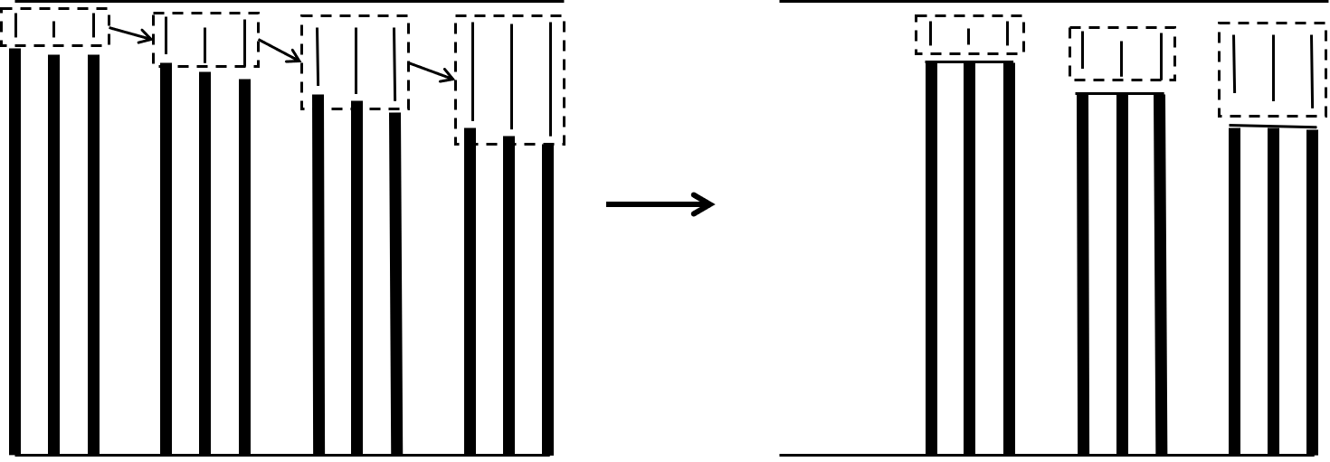
      Heavy items: We apply a rounding and shifting process as follows.

      • $\mathrm{■}$

        Rounding. We adopt the linear grouping scheme from bin packing [10, 25]. Group the heavy items as follows: the first group contains the heaviest $k$ items, the second group contains the next heaviest $k$ items, and so on. Here $k$ is chosen so that the number of groups is constant. We discard the first group (to be compensated later), and round the weight of heavy items in each group to the heaviest item in that group.

      • $\mathrm{■}$

        Shifting. To maintain feasibility, we shift light items groupwise from their groups to lighter ones (where heavy items are lighter).

      This process guarantees that the weight rounding of heavy items is feasible and the total profit loss is bounded. See Figure 1 for an illustration.

   2. (b.2)

      Light items: We show that removing light items of total profit at most $(1/3+\epsilon )$ from each knapsack is sufficient to make the weight rounding feasible. Moreover, we prove that these removed items can be reassembled and packed into the knapsacks in the discarded group created by the heavy-item shifting step.

We guess the critical heavy items, critical light items, non-critical items successively. Our argument follows an “existence-guessing” pattern: before each guessing step, we first prove that there exists a slack solution (containing previously guessed structure); we then guess the assignment of items in this slack solution. The main technical component is the first existence result.

1. 1.

   Existence of a slack solution and its profile. We show that there exists a slack solution whose minimum knapsack profit is at least $\frac{2}{3}-\epsilon$, and whose profile has constant cardinality (Lemma 8). Since the profile has constant size, we can enumerate all possibilities of the profile in polynomial time (Lemma 10).

2. 2.

   Guessing critical heavy items. There exists a slack solution with objective value at least $\frac{2}{3}-2\epsilon$ whose profile is the guessed one (Lemma 13). Moreover, for each rounded type in the profile, every critical heavy item in this solution is heavier than any non-critical heavy item of the same type (Lemma 13). We show that these critical heavy items can be guessed (Lemma 14).

3. 3.

   Guessing critical light items. There exists a slack solution with objective value at least $\frac{2}{3}-3\epsilon$ whose critical heavy items are the guessed ones (Lemma 18). Moreover, for each rounded type of light items, every critical light item in this solution is heavier than any non-critical light item of the same type (Lemma 18). We show that these critical light items can be guessed (Lemma 19).

4. 4.

   Determining non-critical items. Finally, we complete the packing by handling knapsacks with $|I_j|=2$ (Lemma 21) and assigning the non-critical cheap items in knapsacks with $|I_j|\ge 3$ (Lemma 22).

We first show the existence of a slack solution $𝒮$ with $p(I_j)\ge \frac{2}{3}-\epsilon$ for any $j\in [m]$. Then we show the existence of the profile.

Given an optimal solution $(X_1^{\ast },\mathrm{\dots },X_m^{\ast })$ with $p(X_j^{\ast })\ge 1$ for all $j\in [m]$, we convert it into a slack soluton with $p(I_j)\ge \frac{2}{3}-\epsilon$ for any $j\in [m]$. Without loss of generality, we assume every $X_j^{\ast }$ is minimal in the sense that deleting any item makes its total profit less than $1$.

By assumption, each item has profit of at most $\frac{2}{3}-6\epsilon$ and $|X_j^{\ast }|\ge 2$ for any $j\in [m]$. If there exists $j\in [m]$ such that $X_j^{\ast }$ contains two items $i_1,i_2$ with $p(i_1)+p(i_2)\ge \frac{2}{3}-\epsilon$, then we simply set $I_j=\{i_1,i_2\}$. By Definition 5, they are non-critical items and does not affect slackness or the profile.

We thus restrict attention to the case where, for all $i_1,i_2\in X_j^{\ast }$,

We distinguish between the two cases below.

If $w(X_j^{\ast })\le 1-{\epsilon }^3$, then let $I_j=X_j^{\ast }$; by Definition 6, this knapsack is slack, and we are done. Therefore, we assume $w(X_j^{\ast })>1-{\epsilon }^3$ and partition the items in $X_j^{\ast }$ into three sets:

where $w(i)\le 1-{\epsilon }^2$ holds since all items are light,

and

By construction, $X_j^{\ast }=X_e\cup X_c\cup X_d$. If $X_d\ne \mathrm{\varnothing }$, then we can pick any item $i\in X_d$ and set $I_j=X_j^{\ast }\setminus \{i\}$; by Definition 6, we are done. Therefore, we assume that $X_d=\mathrm{\varnothing }$.

Note that there is at most one item in $X_e$, since otherwise there would be two items whose total profit is at least $\frac{2}{3}-\epsilon$, contradicting equation (2). This implies

Let $Y\subseteq X_c$ be obtained by sorting the items in $X_c$ in increasing order of density and adding them until the total weight first reaches at least ${\epsilon }^3$. The set $Y$ always exists due to equation (3), and it follows that

Since $Y$ consists of items with the smallest density, the density of $Y$ is at most the density of $X_c$. Recall that $X_j^{\ast }$ is minimal. Fix any $i\in X_c$. Then , and since $p(i)\le \frac{1}{3}+\epsilon$, we get . Hence, by equation (3) and (4), we have

where the last inequality holds for . Recall that we assume $\epsilon$ is a sufficiently small constant, so the above inequality holds.

Then we let $I_j=X_j^{\ast }\setminus Y$. It is clear that $p(I_j)=p(X_j^{\ast })-p(Y)\ge \frac{2}{3}-\epsilon$ and $w(I_j)=w(X_j^{\ast })-w(Y)\le 1-{\epsilon }^3$, which implies that $I_j$ is slack.

By Definition 4, each knapsack contains at most one heavy item. Denote it by $h$. If $p(h)\le \frac{1}{3}+\epsilon$, let $I_j=X_j^{\ast }\setminus \{h\}$. Then $I_j$ contains only light items, and

By Definition 6, $I_j$ is slack. It remains to consider the case where $p(h)>\frac{1}{3}+\epsilon$.

Let $X_{light}=X_j^{\ast }\setminus \{h\}$. Since $p(h)>\frac{1}{3}+\epsilon$, every item $i\in X_{\mathrm{light}}$ satisfies $p(i)\le \frac{1}{3}-\epsilon$. Otherwise $p(h)+p(i)\ge \frac{2}{3}$, contradicting (2). Recall that by assumption and $w(h)\ge 1-{\epsilon }^2$ by Definition 4. It follows that

Let $Y^{\prime }\subseteq X_{light}$ be obtained by sorting the items in $X_{light}$ in increasing order of density and adding them until $p(Y^{\prime })>1/3$. Let the last item added to $Y^{\prime }$ be $l$, and set $Y=Y^{\prime }\setminus \{l\}$. Recall that every item in $X_{light}$ has a profit of at most $\frac{1}{3}-\epsilon$. We have

Since $Y$ consists of items of the smallest density, its density is at most the density of $X_{light}$. Moreover, by minimality of $X_j^{\ast }$, . Therefore,

The strict inequality follows from (7) and . Finally, equation (6) implies $w(Y)\le w(X_{\mathrm{light}})\le {\epsilon }^2$. Combining the above inequalities yields (5), completing the proof. $\mathrm{⊲}$

We set $I_j=X_j^{\ast }\setminus Y$ where $Y$ is defined in Claim 9. It is clear that $p(I_j)=p(X_j^{\ast })-p(Y)\ge \frac{2}{3}-\epsilon$ and

which implies that $I_j$ is slack.

We have constructed a slack solution $𝒮=(I_1,\mathrm{\dots },I_m)$ with $p(I_j)\ge \frac{2}{3}-\epsilon$ for all $j\in [m]$. Next, we convert $𝒮$ into another slack solution ${𝒮}^{\prime }=(I_1^{\prime },\mathrm{\dots },I_m^{\prime })$ whose profile has constant cardinality.

Consider the knapsacks that contain a heavy item in the slack solution $𝒮$. Let ${𝒥}_H\subseteq [m]$ be the set of indices $j$ such that $I_j$ contains a heavy item. Recall that each such $I_j$ contains exactly one heavy item. We denote it by $h_j$.

We partition ${𝒥}_H$ into groups according to the value of $\lfloor p(h_j)/\epsilon \rfloor$: two indices $j,j^{\prime }\in {𝒥}_H$ are in the same group if $\lfloor p(h_j)/\epsilon \rfloor =\lfloor p(h_{j^{\prime }})/\epsilon \rfloor$. Note that there are at most $1/\epsilon$ such groups since every heavy item has profit at most $\frac{2}{3}-6\epsilon$ and at least $\epsilon$. We handle each group separately as follows.

Fix an integer $t$ and consider the group $𝒦=\{j\in {𝒥}_H\mid \lfloor p(h_j)/\epsilon \rfloor =t\}$. Write $𝒦=\{1,2,\mathrm{\dots },k\}$ after relabeling the corresponding knapsacks, and further relabel so that

For each $j\in [k]$, let $Y_j\subseteq X_j^{\ast }\setminus \{h_j\}$ be the set of light items guaranteed by Claim 9. Recall that $I_j=X_j^{\ast }\setminus Y_j$. We now construct new sets $I_1^{\prime },\mathrm{\dots },I_k^{\prime }$ as follows.

$\bullet$ For $1\le j\le \lfloor \epsilon k\rfloor$, let $\mathrm{\ell }=\lceil \frac{2}{3\epsilon }\rceil$ and define

By Claim 9, each $Y_j$ consists only of light items and satisfies $p(Y_j)\ge \epsilon$ and $w(Y_j)\le {\epsilon }^2$. Hence,

where $\mathrm{\ell }{\epsilon }^2\le \epsilon \le 1-{\epsilon }^3$ holds for . Therefore, $I_j^{\prime }$ is slack by Definition 6.

$\bullet$ For , let $s=j-\lfloor \epsilon k\rfloor$ and set

That is, we replace the heavy item $h_j$ by $h_s$. Since , by equation (8), we have $w(h_s)\le w(h_j)$, and thus $w(I_j^{\prime })\le w(I_j)$.

Note that $\lfloor p(h_j)/\epsilon \rfloor =\lfloor p(h_s)/\epsilon \rfloor$, which implies $p(h_s)\ge p(h_j)-\epsilon$. By Claim 9 and $I_j=X_j^{\ast }\setminus Y_j$, the profit of $I_j$ is

Meanwhile, we have

The first inequality follows from the slackness of $I_j$ in $𝒮$. The last inequality holds since $w(h_s)\le w(h_j)$. By Definition 6, $I_j^{\prime }$ is slack.

Above all, we obtained a slack solution ${𝒮}^{\prime }=(I_1^{\prime },\mathrm{\dots },I_m^{\prime })$. Next, we construct its profile $T$. Let $\delta =\max \{1,\lfloor \epsilon k\rfloor \}$. Let $\{h_{\delta },h_{2\delta },\mathrm{\dots },h_{r\delta }\}$ be the representative heavy items of this group, where $r=\lfloor \frac{k}{\delta }\rfloor =O(\frac{1}{\epsilon })$.

For a group with $\lfloor p(h_j)/\epsilon \rfloor =t$, we set $T_t=\{h_{\delta },h_{2\delta },\mathrm{\dots },h_{r\delta }\}$ to be the set of representative heavy items defined above. Here $1\le t\le 1/\epsilon$ because by assumption, $\epsilon \le p(h_j)\le \frac{2}{3}-6\epsilon$ for any heavy item $h_j$. We then define the profile set $T$ to be the union of $T_t$ over all groups, i.e., $T={\bigcup }_{t=1}^{1/\epsilon }{T}_t.$ Since $r=O(\frac{1}{\epsilon })$ for each group, we have $|T|=O\left({(\frac{1}{\epsilon })}^2\right)$.

It remains to argue that $T$ is the profile of ${𝒮}^{\prime }=(I_1^{\prime },\mathrm{\dots },I_m^{\prime })$. Towards this, it suffices to show that equation (1) holds for each $T_t$ where $1\le t\le 1/\epsilon$. To see this, observe that for each heavy item $h_s\in I_j$ where $s=j-\lfloor \epsilon k\rfloor$, there must exist some $h_{j^{\prime }}\in T$ with $s\le j^{\prime }\le j$, which implies $w(h_s)\le w(h_{j^{\prime }})\le w(h_j)$. Therefore, by equation (4.3), we have

Combined with $\lfloor p(h_{j^{\prime }})/\epsilon \rfloor =\lfloor p(h_s)/\epsilon \rfloor$, we conclude that $T$ is the profile of ${𝒮}^{\prime }$ and $|T|=O\left({(\frac{1}{\epsilon })}^2\right)$. The constructed solution ${𝒮}^{\prime }$ is exactly the solution $𝒮$ claimed in the lemma. $◀$

Since $|T|=O\left({(\frac{1}{\epsilon })}^2\right)$, and according to the definition of profile, every element of $T$ must be one of the heavy items (i.e., at most $n$ possibilities), we can guess $T$ via $n^{O\left({(\frac{1}{\epsilon })}^2\right)}$ enumerations. $◀$

(See the full version of this paper.) $◀$

We first guess the number of critical heavy items of each type in the slack solution $𝒮$ satisfying Lemma 13. Note that the number of heavy-item types is at most $|T|=O({(1/\epsilon )}^2)$. Index these types by ${\tau }_1,\mathrm{\dots },{\tau }_{|T|}$. For each $\mathrm{\ell }\in \left[|T|\right]$, let $n_{\mathrm{\ell }}$ denote the number of critical heavy items of type ${\tau }_{\mathrm{\ell }}$ in $𝒮$, and let $(n_1,\mathrm{\dots },n_{|T|})$ be the count vector. We enumerate all possibilities for $(n_1,\mathrm{\dots },n_{|T|})$. Since $0\le n_{\mathrm{\ell }}\le n$ for every $\mathrm{\ell }$, this takes at most $n^{|T|}=n^{O({(1/\epsilon )}^2)}$ rounds.

Fix the round that guesses the correct tuple. In this round, for every $\mathrm{\ell }\in [|T|]$ we select the heaviest $n_{\mathrm{\ell }}$ items of type ${\tau }_{\mathrm{\ell }}$. Call the union of all selected items $H^{\ast }$. By Lemma 13, the set of critical heavy items used by $𝒮$ is exactly $H^{\ast }$.

We distribute the items of $H^{\ast }$ among $m$ sets $H_1^{\ast },\mathrm{\dots },H_m^{\ast }$, allowing empty sets, so that $|H_j^{\ast }|\le 1$ for all $j\in [m]$ and ${\bigcup }_{j=1}^m{H}_j^{\ast }=H^{\ast }$. We can relabel the knapsacks in $𝒮$ so that property iii is satisfied. Property i and ii follow directly from Lemma 13. $◀$

Note that $H_j^{\ast }$ either contains one heavy item or is empty, meaning that there is no critical heavy item in knapsack $j$.

References

- [1] Yossi Azar and Leah Epstein. Approximation schemes for covering and scheduling in related machines. In Proceedings of the 1st International Workshop on Approximation Algorithms for Combinatorial Optimization (APPROX), volume 1444, pages 39–47. Springer, 1998. doi:10.1007/BFb0053962.
- [2] Nikhil Bansal and Maxim Sviridenko. The Santa Claus problem. In Proceedings of the 38th Annual ACM Symposium on Theory of Computing (STOC), pages 31–40. ACM, 2006. doi:10.1145/1132516.1132522.
- [3] Ivona Bezáková and Varsha Dani. Allocating indivisible goods. ACM SIGecom Exchanges, 5(3):11–18, 2005. doi:10.1145/1120680.1120683.
- [4] Arpita Biswas and Siddharth Barman. Fair division under cardinality constraints. In Proceedings of the 27th International Joint Conference on Artificial Intelligence (IJCAI), pages 91–97, 2018. doi:10.24963/ijcai.2018/13.
- [5] Alberto Caprara, Hans Kellerer, and Ulrich Pferschy. The multiple subset sum problem. SIAM Journal on Optimization, 11(2):308–319, 2000. doi:10.1137/S1052623498348481.
- [6] Alberto Caprara, Hans Kellerer, and Ulrich Pferschy. A PTAS for the multiple subset sum problem with different knapsack capacities. Information Processing Letters, 73(3-4):111–118, 2000. doi:10.1016/S0020-0190(00)00010-7.
- [7] Alberto Caprara, Hans Kellerer, and Ulrich Pferschy. A 3/4-approximation algorithm for multiple subset sum. Journal of Heuristics, 9:99–111, 2003. doi:10.1023/A:1022584312032.
- [8] Deeparnab Chakrabarty, Julia Chuzhoy, and Sanjeev Khanna. On allocating goods to maximize fairness. In Proceedings of the 50th Annual IEEE Symposium on Foundations of Computer Science (FOCS), pages 107–116, 2009. doi:10.1109/FOCS.2009.51.
- [9] Chandra Chekuri and Sanjeev Khanna. A polynomial time approximation scheme for the multiple knapsack problem. SIAM Journal on Computing, 35(3):713–728, 2005. doi:10.1137/S0097539700382820.
- [10] Wenceslas Fernandez de la Vega and George S. Lueker. Bin packing can be solved within 1+ in linear time. Combinatorica, 1(4):349–355, 1981. doi:10.1007/BF02579456.
- [11] Bin Deng and Weidong Li. The budgeted maximin share allocation problem. Optimization Letters, 19(5):955–968, 2025. doi:10.1007/s11590-024-02145-6.
- [12] Leah Epstein and Jirí Sgall. Approximation schemes for scheduling on uniformly related and identical parallel machines. Algorithmica, 39:43–57, 2004. doi:10.1007/s00453-003-1077-7.
- [13] Laurent Gourvès and Jérôme Monnot. Approximate maximin share allocations in matroids. In Proceedings of the International Conference on Algorithms and Complexity (CIAC), volume 10236, pages 310–321. Springer, 2017. doi:10.1007/978-3-319-57586-5_26.
- [14] Laurent Gourvès and Jérôme Monnot. On maximin share allocations in matroids. Theoretical Computer Science, 754:50–64, 2019. doi:10.1016/j.tcs.2018.05.018.
- [15] Dorit S. Hochbaum and David B. Shmoys. Using dual approximation algorithms for scheduling problems theoretical and practical results. Journal of the ACM (JACM), 34(1):144–162, 1987. doi:10.1145/7531.7535.
- [16] John E. Hopcroft and Richard M. Karp. An algorithm for maximum matchings in bipartite graphs. SIAM Journal on Computing, 2(4):225–231, 1973. doi:10.1137/0202019.
- [17] Halvard Hummel. Maximin shares in hereditary set systems. ACM Transactions on Economics and Computation, 13(3):12:1–12:33, 2025. doi:10.1145/3727149.
- [18] Halvard Hummel and Magnus Lie Hetland. Maximin shares under cardinality constraints. In Proceedings of the European Conference on Multi-Agent Systems (EUMAS), volume 13442, pages 188–206. Springer, Springer, 2022. doi:10.1007/978-3-031-20614-6_11.
- [19] Klaus Jansen. Parameterized approximation scheme for the multiple knapsack problem. SIAM Journal on Computing, 39(4):1392–1412, 2009. doi:10.1137/080731207.
- [20] Klaus Jansen. A fast approximation scheme for the multiple knapsack problem. In Proceedings of the 38th International Conference on Current Trends in Theory and Practice of Computer Science (SOFSEM), volume 7147, pages 313–324. Springer, 2012. doi:10.1007/978-3-642-27660-6_26.
- [21] Hans Kellerer. A polynomial time approximation scheme for the multiple knapsack problem. In Proceedings of the International Workshop on Randomization and Approximation Techniques in Computer Science (APPROX), volume 1671, pages 51–62. Springer, 1999. doi:10.1007/978-3-540-48413-4_6.
- [22] Sheng-Yen Ko, Ho-Lin Chen, Siu-Wing Cheng, Wing-Kai Hon, and Chung-Shou Liao. Polynomial-time combinatorial algorithm for general max–min fair allocation. Algorithmica, 86(2):485–504, 2024. doi:10.1007/s00453-023-01105-3.
- [23] Jan Karel Lenstra, David B. Shmoys, and Éva Tardos. Approximation algorithms for scheduling unrelated parallel machines. Mathematical Programming, 46:259–271, 1990. doi:10.1007/BF01585745.
- [24] Barna Saha and Aravind Srinivasan. A new approximation technique for resource-allocation problems. Random Structures & Algorithms, 52(4):680–715, 2018. doi:10.1002/rsa.20756.
- [25] David P. Williamson and David B. Shmoys. The design of approximation algorithms. Cambridge University Press, 2011. URL: http://www.cambridge.org/de/knowledge/isbn/item5759340/?site_locale=de_DE.
- [26] Gerhard J. Woeginger. A polynomial-time approximation scheme for maximizing the minimum machine completion time. Operations Research Letters, 20(4):149–154, 1997. doi:10.1016/S0167-6377(96)00055-7.
- [27] Wenci Yu, Han Hoogeveen, and Jan Karel Lenstra. Minimizing makespan in a two-machine flow shop with delays and unit-time operations is np-hard. Journal of Scheduling, 7(5):333–348, 2004. doi:10.1023/B:JOSH.0000036858.59787.c2.