Multi-Core Integration of Sporadic Events in Time-Triggered Systems

Abstract
Modern safety-critical systems often feature multi-core multi-SoC platforms and execute both periodic and sporadic workloads with real-time requirements. Periodic tasks benefit from a time-triggered (TT) approach, while sporadic events are best modeled by event-triggered (ET) tasks and scheduled using classical online mechanisms such as fixed-priority. Integrating TT and ET tasks in a multi-core environment has mainly been studied in fully partitioned solutions. However, for certain workloads, it may be beneficial to have a global scheduling approach for ET tasks. In this paper, we extend the current state-of-the-art in Response-Time Analysis (RTA) and Real-Time Calculus (RTC) to analyze the schedulability of sporadic ET tasks in a homogeneous multi-core TT system. We generalize previous promising results integrating TT and ET tasks using affine envelopes to homogeneous multi-core systems. While our method can be applied to any TT schedule generation mechanism, we also present a concrete schedule synthesis method based on a variant of the Least-Laxity First scheduling approach. We demonstrate the performance of our approach, in terms of both schedulability and runtime, through real-world and synthetic experiments inspired by real workloads. We note that our affine-envelope-based interference bound and the generalized burst limiting constraint (BLC) are also independent of the concrete TT synthesis algorithm and of the underlying timing analysis method (RTA or RTC). This modularity allows the framework to be combined with alternative schedulability analyses or TT schedule generation techniques, while preserving the demonstrated gains in schedulability and scalability for mixed TT and ET workloads on homogeneous multi-core platforms.
Keywords and phrases:
time-triggered (TT), event-triggered (ET), scheduling, real-time, real-time calculus, response-time analysisCopyright and License:
![[Uncaptioned image]](x1.png) © Anaïs Finzi and Silviu S. Craciunas; licensed under Creative Commons License CC-BY 4.0
© Anaïs Finzi and Silviu S. Craciunas; licensed under Creative Commons License CC-BY 4.0
2012 ACM Subject Classification:
Computer systems organization Dependable and fault-tolerant systems and networksEditor:
Angeliki KritikakouSeries and Publisher:
 Leibniz International Proceedings in Informatics, Schloss Dagstuhl – Leibniz-Zentrum für Informatik
1 Introduction
Modern safety-critical applications often feature multi-core multi-SoC platforms, like those found in automotive systems [45], and execute both periodic and sporadic workloads with real-time requirements. Previous solutions [52, 31, 22, 44] employ a combination of time-triggered (TT) and fixed-priority (FP) scheduling to ensure the deadlines and timing requirements of periodic and sporadic tasks. Using TT scheduling for periodic tasks has the benefit of increased stability, predictability, and compositionality, while simultaneously ensuring low jitter and guaranteed end-to-end latencies in distributed applications that communicate over deterministic backbones (e.g., TSN) [47, 64, 55, 43, 46]. However, TT scheduling is quite inflexible when handling sporadic event-triggered (ET) tasks. For these workloads, FP scheduling allows more flexibility resulting in lower average response times. Hence, many distributed multi-SoC multi-core platforms (c.f. [22, 45]) that have both periodic tasks and sporadic events with complex dependencies (e.g., cause-effect chains [6]) use a TT scheduler for executing periodic tasks according to a statically defined and offline computed schedule table, while a 2nd-level FP scheduler that runs in the idle slots of the static TT schedule dispatches sporadic ET tasks. This solution ensures a deterministic temporal behavior, both in terms of fulfilling complex dependencies for periodic tasks and guaranteeing deadlines for both sporadic and periodic tasks, while not sacrificing flexibility [65, 43, 55, 47, 18].
Traditionally, solutions that integrate sporadic event-triggered (ET) tasks into time-triggered systems, like the ones described in [52, 31, 44, 19], either consider only single-core platforms or employ a fully partitioned approach for both TT and ET tasks. This may lead to lower schedulability and sub-optimal resource usage, especially for ET tasks, for which a global scheduling approach can be more beneficial for certain workloads [12, 4]. Additionally, ET workloads are often bursty and incrementally evolving, making static partitioning impractical, while modern platforms and OSes already rely on global scheduling to maximize flexibility and utilization.
The approach from [19] shows the most promising results in terms of schedulability and runtime for creating TT schedules that respect both TT and ET task deadlines, while employing a greedy heuristic to pre-assign all TT and ET tasks to cores in the offline phase. The approach in [19] begins by expressing a constraint for generating the TT schedule for periodic tasks as a maximal affine envelope. This envelope guarantees that as long as the generated TT schedule respects it in the form of a burst limiting constraint (BLC), all sporadic ET tasks fulfill their deadlines. The BLC can be integrated into any existing TT schedule generation algorithm, and, the authors in [19] use a TT schedule generation method that enforces the BLC via a modified Least-Laxity-First (LLF) scheduler. However, [19] is limited to fully-partitioned systems and cannot be readily adapted to global scheduling. The framework used in [19] does not apply to global scheduling, and the proof of the BLC enforcing the ET deadlines is based on hypotheses of strict partitioning. More generally, global scheduling has more complex patterns of interferences and is more difficult to analyze [28].
In this paper, we tackle these challenges to extend the approach from [19] to global scheduling. For this purpose, we utilize Response-Time Analysis (RTA) and Real-Time Calculus (RTC). Both have been used in numerous research papers [34, 7, 27, 19, 61, 15, 39] to assess timing requirements of real-time tasks. Additionally, RTA and Network Calculus [36] (i.e., the framework from which RTC was developed) were formally compared in [53], providing a strong basis for building a similar model for both methods. However, until now, applying RTA or RTC to a global fixed-priority scheduling with both ET and TT tasks was not a viable solution, due to the pessimism of existing RTC theory and the absence of RTA theory for mixed (i.e. ET and TT) global scheduling.
Hence, the primary contribution of this paper (Section 3.1) is an extension of busy-period computation to system mixing shaped (e.g., TT) and unshaped task (e.g., ET) sets. We then use this new definition to extend both RTA and RTC theories with a method for analyzing the schedulability of real-time tasks (both event- and time-triggered) scheduled using global fixed-priority scheduling on homogeneous multi-core systems. The secondary contribution is the use of our novel RTA and RTC extensions to generate a schedule enforcing ET task deadlines in homogeneous multi-core multi-SoC platforms. In Section 3.2, we propose a global BLC to manage the global multi-core context, and in Section 3.3, we integrate the global BLC to a global LLF scheduler. The BLC is independent of the schedule synthesis method and applies to any synthesis algorithm. We also note that our method can be combined with different RTA formulations, e.g., those in [60] and [14], to further improve schedulability results and accommodate more general task models (i.e., supporting arbitrary deadlines). We evaluate performance in terms of schedulability and runtime, with and without migration overhead, compared to fully partitioned solutions (Section 4). We also empirically characterize RTC’s limitations relative to RTA, highlighting the higher runtime of RTC. Finally, we compare against existing hierarchical scheduling approaches and show improved schedulability and runtime (Section 4.2.4), before concluding in Section 5.
2 Preliminaries
2.1 System model
We assume a platform composed of identical unit-speed processors. The system utilization is at most since this is a necessary condition for the schedulability of real-time tasks [3]. A time-triggered (TT) task dispatcher is executing TT tasks according to a static schedule table that is generated offline. Idle slots within the TT schedule can be used by ET tasks, which are scheduled at runtime by a -level preemptive global fixed-priority scheduler. We consider non-parallel tasks, i.e., ET and TT tasks can only execute on a single core at the same time. We denote the sets of TT and ET tasks by and , respectively. Each TT or ET task is characterized by the tuple , where denotes the worst-case execution time and denotes the relative deadline. For TT tasks, represents the task period, whereas for ET tasks, we consider a sporadic task model in which specifies the minimum inter-arrival time (MIT). Both TT and ET tasks are assumed to have constrained deadlines, i.e., .
The system has a microtick , which is the smallest granularity for scheduling decisions and is usually given by the limits of the hardware and underlying OS. We use discrete time where any time value used for scheduling is a non-negative integer [27]. Similar to [19, 35, 31], the scheduling timeline for TT tasks can be divided into equal segments by the macrotick (also called slot length) [35, 31], which is a multiple of the microtick . We use the macrotick ratio to define the set of slots of a static TT schedule , with each slot (of duration ) being either idle (i.e., can run an ET task) or executing a TT task. The choice of macrotick involves a trade-off between schedulability, system overhead, and schedule synthesis runtime. TT slots are scaled to macrotick to reduce the synthesis search space, whereas ET tasks require microtick granularity to accurately model fine-grained arrival, preemption, and migration behavior. A macrotick equal to the microtick () offers optimal granularity for placing TT slots but can lead to high system overhead and a more complex offline schedule synthesis. In contrast, a higher macrotick reduces the number of TT slots, lowering scheduling overhead, but limits placement options. The choice of macrotick rests with the system designer. We assume that , are correctly scaled to a multiple of the for ET tasks, and to a multiple of the for TT tasks. Idle slots within the TT schedule can be used by ET tasks, which are scheduled at runtime by a -level preemptive global fixed-priority scheduler, with a granularity . Each schedule repeats after the schedule cycle (hyperperiod) , which is a common multiple of the TT task periods (c.f. Sect. 3.3).
In the case of a global scheduling dispatcher, we consider that ET tasks can be migrated at any time, and TT tasks can only be migrated at the start of a TT slot. In the case of fully partitioned multi-core scheduling, both TT and ET tasks are pre-assigned to a core and cannot migrate, even between jobs.
We introduce several notations from [19] to improve readability. For any task , we denote its priority by and its utilization by . The total utilization of all TT tasks is given by , while the total utilization of all ET tasks is denoted by . Following the same notation, we define as the total computation time of all TT tasks. At runtime, as illustrated in Figure 1(a), the dispatcher selects one ready task with the highest priority. All TT tasks are assigned the same priority, which is the highest in the system. ET tasks have lower priority than TT tasks and are ordered according to their relative priorities: if has higher priority than , i.e., , then . We further assume that each ET task has a distinct priority, namely for all .
2.2 Response-Time Analysis
RTA was originally introduced in [34] for constrained-deadline task systems. Here, we use the description from [26]. RTA uses the notion of the level- busy period, defined as the longest continuous interval during which tasks with priority higher than or equal to that of some task execute until the active job of completes. In existing multi-core analyses, the level- busy period of a task consists of three components: 1) the body, which captures the contribution of all jobs whose release times and deadlines both lie within the level- busy period; 2) the carry-in contribution, which accounts for at most one job released before the start of the level- busy period; and 3) the contribution of at most one job released within the level- busy period whose deadline occurs after the end of that period. The workload of a task over a given busy period is the total execution time accumulated by that task within the period. The interference represents the portion of the workload that can actually interfere with , that is, the part that may prevent from executing. We use and to denote, respectively, the workload and interference bounds over an interval of length when has no carry-in jobs. Similarly, and denote the corresponding workload and interference bounds over an interval of length when has carry-in jobs.
In [27, 26] (with processor capacity and unique priority for each ) the total interference on one job of task is:
| (1) |
where denotes the set of all partitions of the higher-priority task set into the subsets and , such that , , and . Maximizing over allows to capture the worst-case total interference under the condition that at most tasks have carry-in jobs, while all remaining tasks have no carry-in. Thus, , which can be computed in linear time, represents the maximum interference generated by higher-priority tasks on a job of during a level- busy period of length .
The interferences and workloads are:
with and the worst-case response time of . Using the above, the following RTA was proposed in [27] for constrained deadlines:
Theorem 1 (2009-RTA-constrained [27]).
Consider a set of tasks and a task such that . Let be the minimal solution of the following Eq. (2) by doing an iterative fixed point search of the right-hand side, starting with .
| (2) |
If such that , , then is an upper bound of the worst-case response time of .
The searches return “unschedulable” as soon as , since .
2.3 Real-Time Calculus
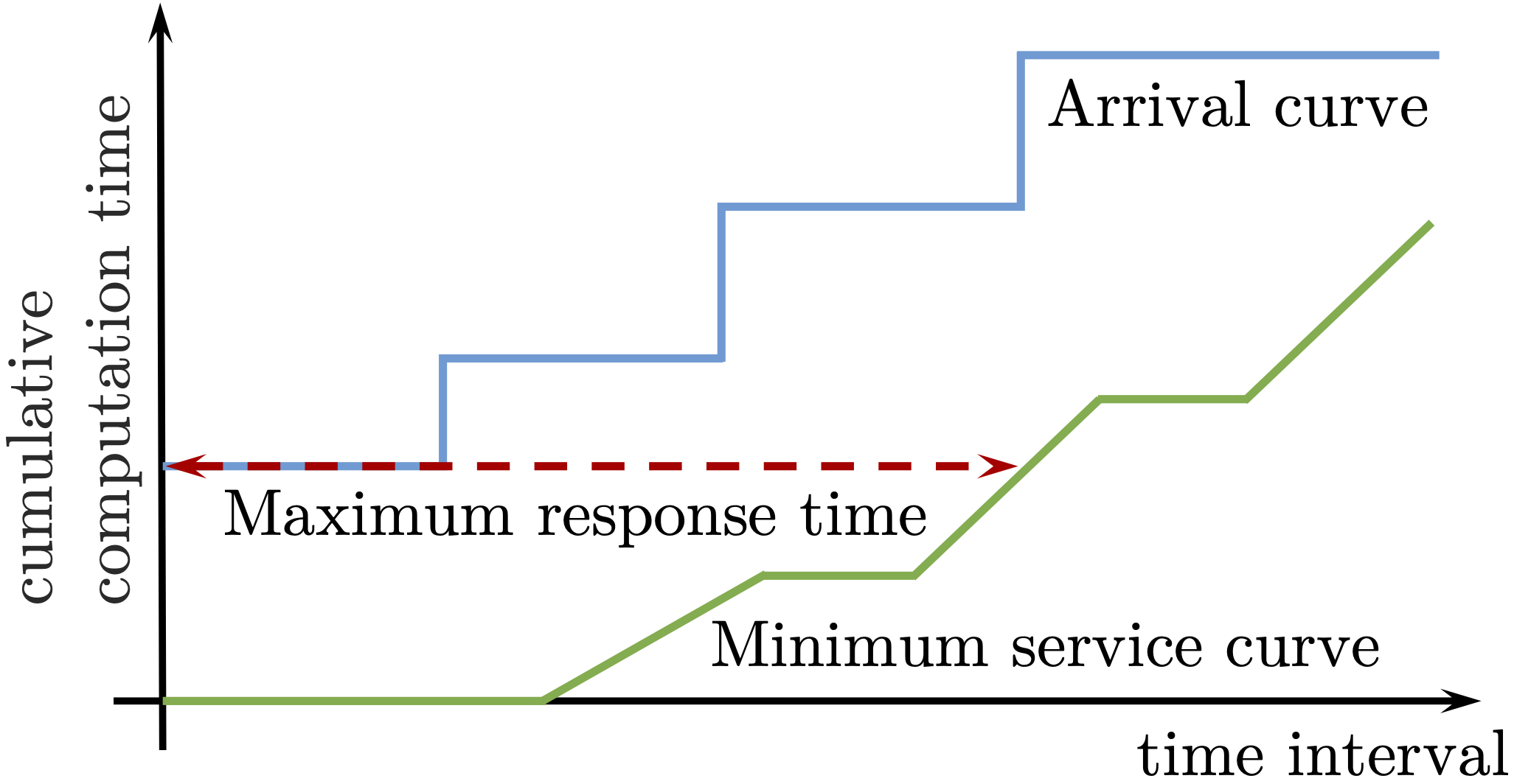
RTC [63] is a framework used to calculate the worst-case response-time (WCRT) of real-time tasks (e.g. [59]). The WCRT of is based on the distance between a curve representing the arrival of requests and a curve representing the service offered. The WCRT is detailed in Theorem 5 and illustrated in Figure 1(b). We refer the reader to [19, 63, 48] for a more complete and detailed description of Real-Time Calculus.
Definition 2 (Arrival curve [63]).
An arrival curve of a request function associated to is a non-decreasing function satisfying: .
An arrival curve denotes the maximum number of requests (which may be in terms of cycles, time units, etc) arriving during an interval .
Definition 3 (Service curves [63, 13, 61]).
A maximum service curve and a minimum service curve of a capacity function associated with a set of tasks are non-negative and non-decreasing functions satisfying: . They can also be defined using the request and output cumulative functions and as follows: , with .
These curves denote the processing power (which may be in terms of processor cycles, time units, etc.) available to from the resource during an interval ]s,e].
Definition 4 (Strict minimum Service curves [63, 13, 61]).
A strict minimum service curve of a set of tasks with an output cumulative function , is non-negative and non-decreasing function satisfying: , backlogged period111a period during which tasks of the given set are waiting to be executed. .
This curve denotes the minimum processing power that will be used by during a backlogged interval ]s,e].
Theorem 5 (Maximum response time [13][36]).
For a dispatcher offering a minimum service curve to with an arrival curve , the WCRT is the maximum horizontal distance222hDev(f,g) = computed between and .
Theorem 5 is not used in multi-core systems. However, the proof in [36] Section 1.4, Theorem 1.4.2 (Delay Bound), shows that they depend solely on the mathematical definition of the curves detailed in Definitions 2 and 4 and so they can be applied to a multi-core system. The challenge of using this theorem in multi-core systems is to compute accurate arrival curves and service curves for the given tasks and dispatchers.
Theorem 6 (Minimum remaining service curve [10]).
For a single-core preemptive fixed-priority task dispatcher offering a strict minimum service curve , to a set of tasks with priorities and arrival curves , a minimum service curve remaining to a task of priority is the non-decreasing positive function 333, with with
Since we will do a per-task analysis, we must model an arrival curve for each task and the service offered by the multi-core system to each task .
If task releases jobs with execution cost according to a period, or minimum inter-arrival time, , then it can be represented by a staircase arrival curve , where and for [9]. Alternatively, it can be upper-bounded by the more pessimistic linear arrival curve , defined by and for , with and [11]. Within a given schedule slot, a task executes at a constant rate , corresponding to one unit of computation per unit of time, after an initial delay, or latency, . This latency may result from blocking caused, for example, by higher-priority tasks. Such behavior corresponds to a rate-latency service [11], which is modeled by the function .
2.4 Related work
Integrating ET and TT tasks has been studied in a holistic approach [51, 52, 50], which uses a greedy method to evaluate TT and ET schedulability. However, this approach is limited to single-core nodes with strictly periodic and non-preemptive TT slots, as well as periodic ET tasks with bounded jitter. In contrast, our method is designed for global multi-core scheduling, supporting a more flexible preemptive, non-strictly-periodic TT task model and sporadic ET tasks. Meroni et al. [47] present simple (SPoll) and advanced polling (Adv Polling) for integrating ET and TT tasks in partitioned multi-core systems. SPoll assigns a polling server to each ET task by oversampling the period to ensure ET schedulability. Adv Polling leverages hierarchical analysis [1, 57, 58, 54] to decouple TT schedule synthesis from ET analysis, using a genetic algorithm to solve the allocation problem. Our method addresses the global scheduling of TT and ET tasks without fixed task allocation.
In multi-core systems, the “critical instant” concept from single-core schedulability analysis does not always hold, and scheduling can exhibit timing anomalies. This makes determining the true worst-case behavior in multi-core systems significantly more challenging than in single-core systems [28]. Several works [42, 32, 56, 8, 38] address multi-core hierarchical scheduling. Resource abstraction models such as the Multi-processor Periodic Resource (MPR) model for virtual clustering [56] and the Bounded-Delay Multipartition (BDM) [42] interface, enable compositional analysis by encapsulating components behind abstract resource interfaces which can be beneficial for integrating TT and ET tasks. However, when used in this context, both TT and ET tasks are encapsulated behind abstract resource interfaces. The initial work in [38] provides a coarse interface (bandwidth only) that is not expressive enough to be able to capture fine-grained TT burstiness. The MPR model specifies a collective budget provided every period with a bounded concurrency . The BDM interface [42] balances total bandwidth and maximum delay for admission control and allocation. When TT tasks are modeled as higher-priority supply, the resulting analysis must conservatively account for their potential parallel execution, which can lead to pessimism for predominantly sequential TT workloads and does not explicitly exploit restricted migration patterns or statically synthesized TT schedules. Moreover, such approaches may be too coarse for tight TT and ET integration. They cannot express fine-grained TT bursts, cannot synthesize TT schedules that explicitly respect ET deadlines, and cannot capture the strong coupling between offline TT synthesis and online ET scheduling that we address. We compare directly to BDM, because, as shown in [42] (Section IV-A), it provides a compositional multiprocessor resource abstraction that remains well-defined without strong synchronization assumptions, unlike MPR. Moreover, BDM is most similar to our BLC envelope definition, i.e., they are symmetric since BDM defines a lower bound on supply while BLC defines an upper bound on demand/interference. In the experiment section (c.f. Section 4.2.4) we show that our method dominates BDM across all evaluated scenarios both in terms of schedulability and runtime.
We build upon [19] where an RTC approach is introduced that expresses a constraint for the TT task schedule (a maximal affine envelope), which ensures sporadic ET task deadlines and models this envelope as a burst limiting constraint (BLC), which can be integrated into any existing TT schedule algorithm. It is shown in [19] that the method outperforms all previous approaches in terms of schedulability and runtime, including Holistic scheduling [51, 52, 50], SPoll [47], Adv Polling [47], and Slot Shifting [23, 30, 29, 31]. However, the work in [19] mainly focuses on the single-core case and only handles multi-core in a fully partitioned variant. The RTC theory used in [19] cannot be applied to global scheduling, and the BLC is only defined for a single core, its proof is based on hypotheses of strict partitioning. In this paper, we extend not only the RTC and RTA theory but also the approach from [19] to be able to handle a global scheduling approach for multi-core systems.
Finally, extending RTC to multi-core systems was studied in [39], where a pseudo-polynomial-time algorithm for testing response times of task jobs was proposed. However, [39] only considered ET tasks.
2.5 B3LF and LMminB3LF
In [19], two methods (called B3LF and LMminB3LF, c.f. Figure 2) are presented to compute TT schedules that not only ensure the schedulability of TT tasks but also fulfill the ET deadline constraints. Both methods from [19] share the same two key functions: 1) they compute a schedule enforcing a Burst Limiting Constraint (BLC) [19], using a modified Least Laxity First (LLF) scheduler [40]; and 2) perform a schedulability analysis, based on a formal timing analysis using RTC, of the ET tasks.
The BLC shapes the TT schedule to ensure the TT cumulative computation time remains below an affine envelope , with the cumulative rate of the TT tasks, . Depending on the method, the value of is computed differently.
In the case of B3LF (c.f. Figure 2), a binary search is used to compute a maximum TT burst , i.e., the maximum impact that the TT tasks may have on the ET tasks, such that the ET tasks still fulfill their deadlines. Then a schedule enforcing a BLC parameterized with is generated. In the case of LMminB3LF (c.f. Figure 2), a binary search is used to vary the possible used to parameterize the BLC, to find the minimum such that a TT schedule can be generated. Hence, the final TT schedule is computed to have the least impact on ET tasks. Then, using this , the RTC analysis is run to check ET schedulability. If this is not the case, the system is not schedulable.
In the single-core and fully-partitioned multi-core results from [19], LMminB3LF has a similar schedulability to B3LF, with a loss of a few percent in some cases due to different binary searches. However, LMminB3LF offers interesting optimization to maximize schedule re-utilization. In the event of modifications to ET tasks (TT tasks remain unchanged), only the schedulability analysis needs to be run to determine if the generated TT schedule is still valid. In the next section, we will extend both methods to global multi-core systems.
3 ET and TT integration in multi-core systems
As presented in Section 2.5, there are two key parts to B3LF and LMminB3LF: 1) schedulability analysis of the ET tasks; 2) generating a schedule enforcing an affine constraint. We will present these two functions below.
3.1 Schedulability analysis of the ET tasks
Analyzing the schedulability of an ET task often implies calculating the busy-period for any time interval [5, 4, 27], i.e., the maximum interval during which cannot be executed. In this paper, we show how to extend the busy-period computation to integrate the shaping of the TT schedule.
Theorem 7 (Upper workload bound of (r,b)-shaped tasks).
Let a set of tasks be defined by an arrival process shaped by the affine function . An upper bound of the workload of in any interval is .
Proof.
By definition of the shaping of the arrival process, we know that in any interval , the workload is: . Hence, .
We use this to extend the results in [27] to shaped tasks:
Theorem 8.
(Multi-core upper bound of the total interference when mixing unshaped and (r,b)-shaped tasks) Let be a task with priority . Consider a set of tasks with priorities defined by an arrival process shaped by the affine function . Consider a set of unshaped tasks with priorities , with .
The upper bound of the total interference on a job of task , during an interval of duration is:
where is the set of all partitions of the set of tasks of priority higher than into and such that and and .
Proof.
From Eq. (1) and [27], we know that the upper bound on interference due to tasks in is . We know from Theorem 7 that is an upper bound of the workload of , and so, an upper bound of the interference of on . Hence, the sum of these two parts is an upper bound of the total interference on .
Corollary 9.
Let be the set of TT tasks with the same priority and the set of ET tasks with unique priorities (). Let be defined by an arrival process shaped by the affine function . The upper bound on the total interference of one job of during an interval of size , is:
| (3) |
where is the set of all partitions of the set of ET tasks of priority higher than into and such that and and .
Proof.
This corollary is a direct application of Theorem 8.
As in [27], can be computed in linear time, since it is also sufficient to find the maximal values of the difference .
There is a pessimistic aspect to the proposed method: the workload is evenly divided among the different cores, with no consideration for the non-parallelism of the tasks. We considered that the current task of interest can only be executed on one core at a time to avoid both optimism and over-pessimism. However, we are unable to consider this constraint for the other tasks that impact the task of interest. Consequently, the busy period (i.e., initial waiting time) is maximized, and the overall duration during which at least one core is idle is minimized. However, this also means that our proposed method is not affected by the timing anomalies present in fixed-priority preemptive multi-core scheduling that arise from the relative priority order of higher-priority tasks (cf., for example, Observation 4 in [2]).
It is important to note that we do not bind the service to a specific core, but rather constrain the ET tasks to use only one core at a time; thus, ET migration remains possible. Without the possibility of migration, an ET task would always be assigned to a specific core (fully partitioned model) and would be impacted by higher-priority tasks assigned to the same core, also without the ability to migrate, in a way not taken into account by this model.
In the next part, we will present how the total interference can be used to calculate the worst-case response time with two formal timing analysis methods: RTA and RTC.
3.1.1 Response-Time Analysis in multi-core systems
The Response-Time analysis of an ET task in a multi-core system with both TT and ET tasks is a direct application of either Theorem 1, with defined in Corollary 9.
Because the worst-case response time is part of the definition of , the analysis must be done in decreasing order of priority, so that of higher priority is known.
3.1.2 Real-Time Calculus analysis in multi-core systems
As the ET tasks are known, is known. Only the service curve of the ET tasks denoted needs to be computed to apply Theorem 5. Since the same task cannot run on multiple cores simultaneously, the existing RTC theorems cannot be applied directly without introducing significant pessimism to the result. The main reason is that the current RTC theory (i.e., Theorem 6) does not bind a task to only use one core at a time. If we directly apply Theorem 6, all tasks of higher or equal priority than the task of interest will be considered in the service curve, which leads to pessimism. We either consider that the task of interest can use only one core, i.e., , and be very pessimistic since some of the other tasks may execute on other cores and have no impact, or consider that the task of interest can use all cores, i.e., and be too optimistic (and have an invalid practical model). Additionally, [4] showed that the periodic case is not the worst-case for asynchronous tasks. So with Theorem 6, only the more pessimistic linear arrival curves and service curves can be safely used in the multi-core context, rather than the staircase functions.
In Theorem 10, we use the newly defined upper bound of the interference in a multi-core system to define a new strict minimum service curve, which can be used in Theorem 5 alongside staircase arrival curves to compute the delay bounds.
Theorem 10 (Strict minimum service curve).
Let be a set of ET and TT tasks, with TT tasks having the same priority and each ET task has a unique priority .
Let be an upper bound of the total interference of tasks of priority higher than on a job of task . A strict minimum service offered to an ET task of priority , denoted , is such that and , .
Proof.
By definition, is an upper bound of the busy period and can prevent from running on a core during an interval of length . In the case where multiple cores are available, the maximum time all the cores can be blocked is . Hence, in an interval of length , the minimum duration when at least one core is available to execute is . Additionally, the duration when a core is available cannot be negative and cannot decrease when the considered interval increases. Hence, backlogged interval , the delta of the output cumulative function between and , is such that , according to Definition 4.
We observe a limitation noted in [53] regarding the Network Calculus model, which is also present in RTC: the NC model of flow lacks a notion of individual packets or jobs, and for RTC, there is no notion of individual tasks or jobs.
3.2 Generalizing Burst Limiting Constraint (BLC) to multi-core systems
We have shown that the workload of higher priority tasks used in RTA and RTC depends on the shaping function , the affine envelope the schedule must enforce before the fixed-priority online scheduler. The rate of the affine function is always , the value of depends on the method, B3LF or LMminB3LF (c.f. Section 2.5).
In the next part, we analyze the Burst Limiting Constraint to demonstrate how to parametrize it to shape the TT task workload accurately. The proofs are based on the RTC framework, but could be done using another formalism.
According to Definition 2, an arrival curve is defined by: , . It means that any curve such that is also a TT arrival curve.
Similar to [19], the schedule is the output of the modified LLF scheduler, which itself depends on the BLC. Thus is limited by a maximum service curve of the B3LF , which is the minimum of maximum service curves of the BLC and mLLF :
So, a TT arrival curve in the online fixed-priority scheduler, , is constrained by: We know from [19] that the lower bound of the maximum service offered by the LLF scheduler is , which cannot be used to enforce an affine envelope, as this is the maximum service the multi-core system can offer.
Additionally, since and due to Definition 2, is an arrival curve for TT tasks. By setting the BLC such that , we will be able to create a schedule enforcing the desired TT burst .
Therefore, we must first extend the definition of the BLC from [19] to multi-core systems and define the corresponding . Then we must find the correct parameters for the BLC, i.e., its maximum level and its rate .
Definition 11 (Global Burst Limiting Constraint).
A slot reserved for TT in a TT schedule is invalid under the Burst Limiting Constraint (BLC) if the budget is strictly smaller than at the end of the slot, with the budget behavior:
-
the budget is a continuous piecewise linear function of the time t ,
-
the rate of the budget at time t, , is either the sum of the rates due to the slot of each core : , if the budget is strictly smaller than a maximum value or if , or else the budget remains constant at , i.e., ,
-
when a slot is reserved on core for TT in , the budget decreases at a rate due to ,
-
when a slot is idle on core in (i.e., not assigned to TT on core ), the budget increases at a rate , due to ,
-
is the processing capacity of a core: ,
-
at time , the budget is , i.e. .
We now present the maximum service curve offered to TT tasks by the generalized BLC, which we will use afterwards to parameterize the affine envelop .
Theorem 12 (BLC maximum service curve).
A maximum service curve of a set of TT tasks scheduled on a multi-core system with cores, validated by the Burst Limiting Constraint (BLC) defined in Definition 11 is
Proof.
As with the single-core BLC [19], the proof is based on the proofs from [21, 20] for the Burst Limiting Shaper (BLS) [25, 62] in TSN networks. We denote the computation capacity function offered to TT tasks on all cores, and its variation during an interval , and (to help with the readability of the proof) the processing capacity of one core (in computation units per time unit). According to Definition 3, we search for such that .
We assume a given TT schedule for a multi-core platform with cores. When satisfies the BLC, the corresponding budget is guaranteed to be non-negative, i.e., for all . Moreover, the budget cannot stay at zero: whenever it reaches , the next slot must be idle in order to satisfy the BLC, which causes the budget to increase. Thus, the budget can evolve in only three ways:
-
it increases during an idle slot, provided that its current value is strictly below ;
-
it decreases whenever a slot is allocated to TT in ;
-
it remains saturated at when the slot is idle and the budget has already reached .
Accordingly, we define as the number of computation units over which the budget is saturated at .
We present a lemma related to budget saturation at the maximum level and necessary for the proof of the max service curve. In Lemma 13, we demonstrate how to bound the sum of the budget consumed and the budget gained, depending on the level of budget saturation.
Lemma 13 (Continuous budget bounds).
set of assigned TT tasks fulfilling a BLC, , the variation of the computation capacity is bounded by:
Proof.
Each TT slot causes a decrease of (slot duration is ) of the BLC budget. Each idle slot causes an increase of of the BLC budget. In an interval , for any set of assigned TT tasks fulfilling the BLC, represents the sum of the duration of the TT slots when considering all cores, represents the saturation duration on a single core, represents the sum of the interval time of all cores.
Consequently, the accurately consumed budget is the duration corresponding to the sum of the time of the assigned TT slots in all cores multiplied by the signed TT slope:
Conversely, the gained budget is the duration of the idle slots in all cores: minus sum of the time of the saturated slots for all cores , multiplied by the idle slope. So, is:
Thus , using the fact that , the sum of the gained and consumed budget, i.e., , is: Since the budget is a continuous function with lower and upper bounds and , the sum of the consumed and gained budget is always bounded by and :
Returning to the proof of Theorem 12, we know from Lemma 13:
Thus, We know by definition that: . Hence, we obtain
Therefore, to shape the TT task workload and enforce the ET schedulability, we define: . This gives the following BLC parameters: .
3.3 Integrating the BLC to a task scheduler
The proposed method can be applied to any TT schedule generation method. The TT synthesis algorithm only needs to be able to keep track of the budget and remove the tasks not fulfilling the BLC from consideration until the budget is sufficient again. There are many options for generating TT schedules based on the definition and requirements of TT tasks (e.g., [49, 45, 17]). Any of these algorithms can be adapted to include our BLC constraint and also fulfill ET task deadlines. In this paper, we adapt an LLF-based TT schedule generator. Least Laxity First(LLF) [40] is an online algorithm that uses the current task laxity to assign dynamic priorities to task jobs. LLF has good performance on multi-core systems [37] and is well-suited to track the BLC budget consumption and replenishment at any instant on the discrete timeline [19]. Simulating LLF, or other online algorithms like EDF, to generate TT schedules has been introduced before [16, 44]. However, any work-conserving algorithm will not result in the schedulability of TT tasks and the fulfillment of the BLC, since sometimes it may be necessary to insert idle times even though there are TT tasks with execution time left in order to have the full burst later. For a more in-depth explanation, we refer the reader to the counterexample and detailed description in Figure 4 in [19].
3.4 Global scheduler
The B3LF is detailed through two algorithms which are inspired by and largely follow the algorithms from [19]. Algorithm 1 presents the TT schedule generation under the BLC. The schedule must be valid for any time interval: it is generated for a hyperperiod and must be valid under the BLC indefinitely. It means that the budget variation during the time interval must be positive or null: the budget at the end of the hyperperiod must be greater or equal to the budget at the start of HP so that the budget always remains greater than or equal to . Algorithm 2 shows how to incorporate the BLC into a modified LLF for multi-core.
In Algorithm 1, following an approach similar to [19], we first verify the two sufficient conditions in lines 3 and 9. This verification is performed using our mLLF scheduler through the function mLLF(), which generates a schedule based on the specified initial budget. If these conditions are not satisfied, the mLLF scheduler is executed with different initial-budget values, as shown in line 13, starting from an initial budget equal to the budget at . To reduce the search space we use a similar method as in [19] where we select (line 14) the new initial budget as a multiple of (and not directly ) since this has a large performance boost without sacrificing too much schedulability (c.f. [19]). Similar to [19], Algorithm 1 finishes when a solution is found (i.e., ), or when the final budget reaches the minimum final budget possible, . The function of the final budget is strictly decreasing from one iteration to the next when no solution is found, which ensures the algorithm always finishes.
Algorithm 2 details a multi-core LLF enforcing the BLC. Over all time slots of the hyperperiod, firstly, for each TT task, we check if a deadline has been missed, then we update the remaining duration of the task and update the deadline, if necessary. Finally, the laxity of the TT task is computed. Secondly, we assign the slots for each on each core. After each assignment, the budget is updated before the assignment on the next core. Hence, the BLC is always fulfilled on all cores . Additionally, in the function returning the valid task with the least laxity, i.e., the LL function, see line 11, we check and select only a task that has not been assigned to a core at the current time . In Algorithm 2, contrary to the single-core algorithm (i.e., Algorithm 2 [19]), as idle slots can be scheduled at each time at the same time TT slots are scheduled on other cores, we found no advantage in varying the idle task laxity. Its laxity is set to , to be used if no other task is available and fulfilling the BLC.
4 Experiments
In Section IV in [19], multi-core fully-partitioned solutions were compared. B3LF and LMminB3LF were shown to be the best solutions in terms of synthesis time and schedulability ratio compared to Advanced Polling (Adv Polling) [47], Simple Polling [47] and Slot-Shifting [29, 31], in this order. We now assess the performance of the two Global solutions developed in this paper, i.e., Global B3LF and Global LMminB3LF. We compared them to the 3 best existing solutions as determined in [19], i.e., Fully-Partitioned B3LF, Fully-Partitioned LMminB3LF, and Fully-Partitioned Adv Polling.
For the Fully-Partitioned solutions, we compared several bin-packing algorithms [33], e.g., Best-Fit, First-Fit-Decreasing, Laxity-Round-Robin used in [19], Worst-Fit-Increasing and Worst-Fit-Decreasing (we sort blindly with regard to ET vs. TT). We concluded that all the bin packing which fit as many as possible to the same bin before trying a new one will not work for our problem since, as shown in Section IV in [19], better results are obtained for lower utilization rates in individual bins. Finally, Worst-Fit-Decreasing proved to be better on average than the other options. So in this paper, we assign the tasks to a partition using the Worst-Fit-Decreasing method in which the tasks are sorted in decreasing order with regards to the task rates, then place each item into the bin (i.e., partition) with the minimum load.
We implemented Adv Polling as described in [47, 19] searching through polling task periods with values within . The computation time is set to , as described in [47]. As noted in [19], we can use the efficient utilization-based test for every candidate since TT tasks (and the polling task) have implicit deadlines. We also use an LLF schedule simulation over all TT tasks and including the polling task for Adv Polling to generate the static TT schedule table as described in [47, 19].
We also compare RTA B3LF and RTA LMminB3LF against a multicore version of AdvPoll (AdvPollBDM) that adopts the Bounded-Delay Multipartition (BDM) interface model proposed in [42]. We do not compare to MPR [56] since BDM is superior to MPR as explained in [42] (Section IV-A), and because BDM is most similar to our BLC envelope definition. The core idea is to abstract ET tasks behind a virtualized platform defined by the BDM interface. We set number of physical cores to be equal to the number of physical cores () and derive the bandwidth-optimal BDM interface (, , ) by performing a grid search over feasible values, and for each solving a MILP (using COIN-OR Branch and Cut solver [24, 41]) with the optimization objective to minimize the total bandwidth . Once the bandwidth-optimal BDM interface for ET tasks is determined by selecting the that yields the smallest feasible , TT tasks are allocated to the remaining capacities on the physical cores using a Best-Fit Decreasing strategy. Finally, we use LLF to generate the TT schedule on each core.
All algorithms are implemented in Python, and all experiments were run on a 12th Gen Intel Core i7-1265U ( GHz) processor with 32GB RAM.
4.1 Real world test case
We use the real-world automotive use-case from [19], featuring a core platform. There are tasks with periods , a distribution of and total system utilization of . In the original use-case, all tasks were defined as time-triggered and were pre-assigned to the cores. In [19], the TT tasks are changed to ET when the task’s laxity (i.e., ) is bigger than macroticks, hence converting tasks from the original TT type to be ET. For each resulting ET task the priority is computed as . TT tasks with laxity under macroticks are kept of type TT, with priority set to . Then, each ET task priority is increased until each ET task has a unique priority. We used and and so .
All assessed methods successfully computed schedules for all cores. The runtimes are as follows: ms for RTA Global B3LF, ms for RTA Global LMminB3LF, s RTC Global B3LF, s for RTC Global LMminB3LF, ms for Fully-Partitioned B3LF, ms for Fully-Partitioned LMminB3LF, ms for Fully-Partitioned Adv Polling. Unsurprisingly, we can see that RTA is much faster (over 2000 times) than RTC. This is because RTC must calculate each point of the minimum service curve and the arrival curve, whereas RTA converges much faster with the fixed-point search.
4.2 Analysis of synthetic test cases
We created synthetic test cases that align to the macrotick, period distribution, and period values of the real-world use-case. We set the macrotick to and periods are respecting a distribution of .
For each synthetic test set, we generate TT and ET tasks per core. This gives us a total of tasks when considering the 6-cores use-case, which is the number of cores and tasks in the real-world use case. We study constrained deadlines for ET tasks, with . TT tasks have implicit deadlines, i.e., . For each case, we generate individual test sets per tuple (,), with and varying in {0.1, 0.2, 0.3, 0.4, 0.5, 0.6, 0.7} and such that . For each tuple (,), these test sets are merged depending on the number of cores (e.g., for the 6-core use-case, we obtain merged sets for each tuple).
4.2.1 Comparing RTA and RTC
Due to the computation time of RTC, we only computed the results of and for RTC. We found that for constrained deadlines, the schedulability of RTC B3LF (resp. LMminB3LF) is identical to RTA B3LF (resp. LMminB3LF). Concerning the runtimes, RTC is up to 1000 times slower than RTA. Global RTC outperforms fully-Partitioned B3LF for moderate loads (below 50%). For the remainder of the performance analysis, we will focus on the RTA model.
4.2.2 Comparing RTA Global Scheduling and Fully-Partitioned Scheduling
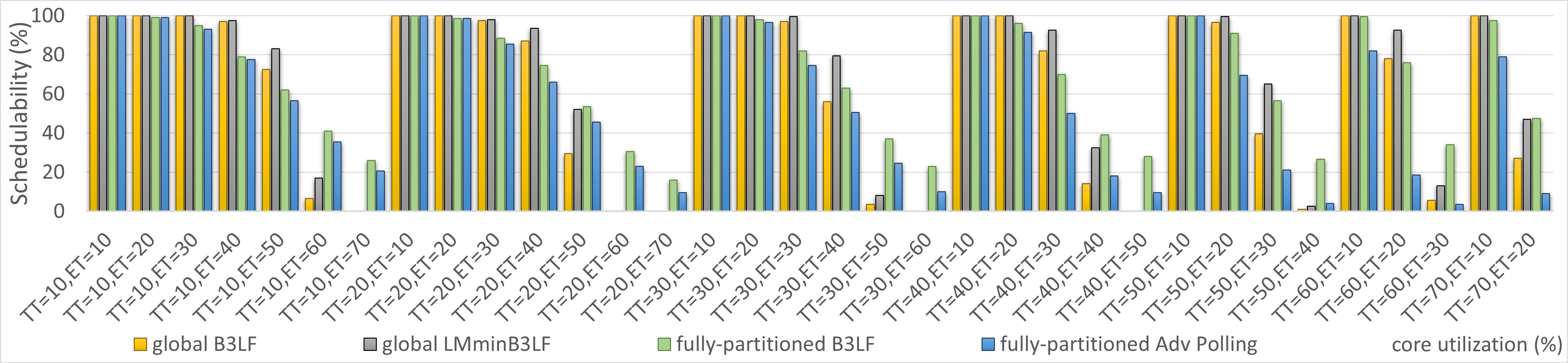
In Figure 3, the schedulability of the methods for (with the exception of ) is as follows: Global LMminB3LF Global B3LF Fully-Partitioned B3LF Fully-Partitioned Adv Polling. For larger utilizations, Fully-Partitioned B3LF is better than Global LMminB3LF and Global B3LF.
The degradation of Global scheduling compared to Fully-Partitioned scheduling is most pronounced for constrained deadlines at high system utilizations, where interference increases, but deadlines remain fixed. It leads to a rapid loss of schedulability once worst-case interference exceeds the deadline. More fundamentally, sources of pessimism affect the global analysis:
-
1.
the separation of TT and ET interference (c.f. Theorem 8): to obtain safe bounds under Global Scheduling, TT and ET interference must be accounted for separately, which is conservative and leads to larger worst-case interference bounds than per-core analyses.
-
2.
The use of a single global BLC: Fully-Partitioned scheduling benefits from multiple local BLCs, which yield tighter bounds. Global scheduling necessarily relies on a single global BLC, which is inherently more pessimistic.
-
3.
The assumption of having an even workload distribution: the analysis evenly distributes workload across cores and does not exploit task non-parallelism. This maximizes busy periods and minimizes idle intervals, further increasing pessimism.
Additionally, we notice that contrary to the Fully-Partitioned case [19], for Global Scheduling, B3LF has a much larger run time than LMminB3LF (e.g., 1322 ms vs. 360 ms on average for Global Scheduling). This shows that the binary search takes more time for the formal timing analysis (i.e., RTA) than the scheduling algorithm in the case of Global Scheduling. It was the opposite for Fully-Partitioned scheduling. This again highlights the differences of approaches between Global Scheduling and Fully-Partitioned scheduling, in particular the increased complexity of the interference patterns in Global Scheduling.
Note that the Global LMminB3LF has a relatively larger run-times (360 ms on average) than the Fully-Partitioned Adv Polling (255 ms on average) and relatively larger run time than Fully-Partitioned B3LF (322 ms on average) and LMminB3LF (119 ms on average).
4.2.3 Comparing RTA B3LF and RTA LMminB3LF
We continue our performance evaluation with a more in-depth comparison of RTA B3LF and RTA LMminB3LF. In Figure 3, we can see that B3LF is marginally worse than LMminB3LF for Global Scheduling for constrained deadlines. On average, over all the tested scenarios (i.e., and varying in {0.1, 0.2, 0.3, 0.4, 0.5, 0.6, 0.7} and such that ), for constrained deadlines, the schedulability of LMminB3LF is , while the schedulability of B3LF is only .
4.2.4 Comparing global B3LF and BDM
We ran the same suite of experiments over 6 cores as in Figure 3 and show the comparison in Figure 4. For this experiment, we set both macrotick and microtick to since BDM does not easily support different time granularity for different interfaces. As can be seen both RTA-based B3LF and LMminB3LF are better than AdvPollBDM in terms of schedulability (left y-axis) and by to orders of magnitude in terms of runtime (logarithmic right y-axis) in all test cases. We note that our implementation of AdvPollBDM is bandwidth optimal but not allocation or feasibility optimal. In [42] the authors show that for a given ) there may be multiple interfaces that all satisfy schedulability but differ in structure (concavity, distribution of , allocation flexibility). It may be that sub-optimal BDM interfaces with slightly larger could be better from the perspective of TT task allocation and schedule generation. We leave solving the optimality of BDM in terms of global schedulability for future work.
4.2.5 Impact of migration on RTA Global Scheduling
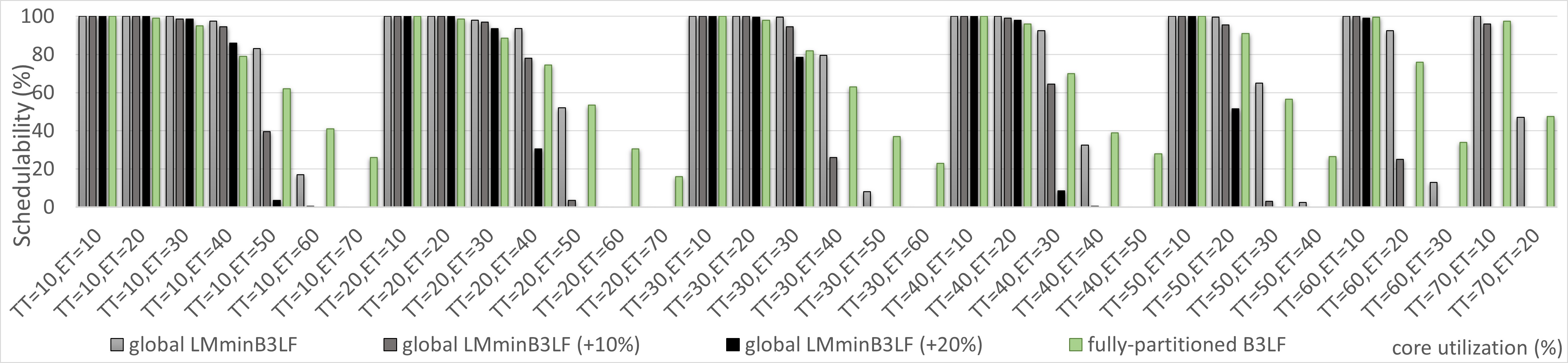
Here, we focus on Global LMminB3LF since it has the best schedulability in most use-case. Runtime, while important, is not as central as schedulability, since we perform offline, rather than online scheduling of real-time systems. We have shown in the previous sections that Global Scheduling has better schedulability than the other methods for total loads lower than 70%. However, depending on the implementation, the migration of tasks can lead to additional delays that need to be factored into the task duration. Since the migration overhead depends on the hardware and implementation of the multi-core system (e.g., L1/L2 cache, memory bus, OS), we consider different migration impacts. Depending on their setup, users can look up the appropriate results to assess which has the best potential for improvement in their case. We consider the impact of migration M by defining the new duration , for all TT and ET tasks in the case of Global Scheduling.
We present the results obtained for the constrained deadline use-cases in Figure 5. We can see that, as expected, increasing the impact of migration decreases the schedulability of the Global B3LF.
For M=0%, we showed that Global LMminB3LF (resp. B3LF) is better for . For M=10%, Global LMminB3LF (resp. B3LF) is generally better for . For M=20%, Global LMminB3LF (resp. B3LF) is generally better for .
Hence, the best solution between the Global and Fully-partition solutions compared here depends on the load of the system and the impact of migration.
4.2.6 Comparing different numbers of cores
| = 2 | = 4 | = 6 | = 8 | = 12 | |
|---|---|---|---|---|---|
| Global B3LF | 82.6% | 67.1% | 61.5% | 58.6% | 54.8% |
| Global LMminB3LF | 85.5% | 71.9% | 66.8% | 63.7% | 60.2% |
| Fully-Partitioned B3LF | 91.2% | 76.7% | 68.5% | 61.1% | 53.4% |
| Fully-Partitioned Adv Polling | 83.7% | 65.6% | 56.5% | 50.2% | 43.2% |
To finish our performance evaluation, we vary the number of cores. The results are presented in Table 1. When comparing the evolution of schedulability for a number of cores , we can see in Table 1 that the average schedulability decreases when increases, for all studied methods. For , the average schedulability of the Global solutions remains slightly lower than the average schedulability of the Fully-Partitioned B3LF. Fully-Partitioned B3LF is generally better than the Global solutions for . However, for , the average schedulability Global B3LF (resp. LMminB3LF) is better than the average schedulability of the Fully-Partitioned B3LF. The average schedulability of both Global solutions is always better than the average schedulability of the Fully-Partitioned Adv Polling. Hence, it seems that the advantage of implementing one of the Global Scheduling solutions compared to Fully-partitioned B3LF increases with the number of cores. Fully-Partitioned scheduling statically binds each task to a single core. When increasing the number of cores, fragmentation increases, making the system harder to schedule. However, Global scheduling allows tasks to execute on any core and so it not as negatively impacted by the increased fragmentation.
While partitioned scheduling may outperform global scheduling at high utilization for a fixed number of cores, its scalability with respect to core count is worse. This is an important tradeoff for practical systems where increasing complexity is leading to to a higher number of cores. Additionally, when increasing the number of cores, Global scheduling also has the advantage of not requiring the new computation of the task-to-core assignment a fully-partitioned system does.
5 Conclusion
We have studied the problem of integrating event-triggered (ET) tasks into uniform multi-core time-triggered (TT) systems. We introduced a unified analytical framework that combines an extension of busy-period computation with affine shaping of TT workload, enabling both Response-Time Analysis (RTA) and Real-Time Calculus (RTC) to handle mixtures of shaped (TT) and unshaped (ET) tasks. Based on this analysis, we generalized the Burst Limiting Constraint (BLC) to the multi-core context and integrated it into a global Least-Laxity-First (LLF)-based TT schedule synthesis algorithm.
Our experimental evaluation demonstrates the benefits of the proposed global approach. In the real-world automotive case study, all global methods successfully generated valid schedules. We have also identified a gap of more than three orders of magnitude between the runtimes of the RTA-based and RTC-based variants. Across the synthetic experiments, the global RTA-based B3LF and LMminB3LF consistently achieved higher schedulability than the BDM-based AdvPollBDM approach for all evaluated utilization combinations, while also improving runtime by one to two orders of magnitude. Compared to fully partitioned methods, the global variants demonstrated clear schedulability advantages, reflecting the benefit of avoiding static task allocation, generally for loads up to 70%, and in some cases, for loads up to 80%. These results underline the advantage of explicitly coupling offline TT synthesis with online ET analysis through a global affine envelope, rather than relying on resource abstraction or strict partitioning.
The RTA analysis we use in this paper is pessimistic for constrained deadlines and optimistic for arbitrary deadlines [60]. We note that our method is not tied to a specific RTA formulation. We can integrate any suitable analysis technique, for example, those in [60] and [14], to further improve schedulability results and accommodate more general task models (i.e., supporting arbitrary deadlines). We plan to investigate these extensions in future work.
References
- [1] Luis Almeida and Paulo Pedreiras. Scheduling within temporal partitions: Response-time analysis and server design. In Proc. EMSOFT, 2004. doi:10.1145/1017753.1017772.
- [2] Björn Andersson and Jan Jonsson. Some insights on fixed-priority preemptive non-partitioned multiprocessor scheduling. In Proc. RTSS, 2000.
- [3] Theodore P. Baker and Michele Cirinei. A necessary and sometimes sufficient condition for the feasibility of sets of sporadic hard-deadline tasks. In Proc. RTSS, 2006. doi:10.1109/RTSS.2006.7.
- [4] Sanjoy Baruah. Techniques for multiprocessor global schedulability analysis. In Proc. RTSS, 2007. doi:10.1109/RTSS.2007.35.
- [5] Sanjoy K. Baruah, Louis E. Rosier, and Rodney R. Howell. Algorithms and complexity concerning the preemptive scheduling of periodic, real-time tasks on one processor. Real-Time Syst., 2(4), 1990. doi:10.1007/BF01995675.
- [6] Matthias Becker, Dakshina Dasari, Saad Mubeen, Moris Behnam, and Thomas Nolte. End-to-end timing analysis of cause-effect chains in automotive embedded systems. Journal of Systems Architecture, 80(C), 2017. doi:10.1016/j.sysarc.2017.09.004.
- [7] Marko Bertogna and Michele Cirinei. Response-time analysis for globally scheduled symmetric multiprocessor platforms. In Proc. RTSS, pages 149–160. IEEE, 2007. doi:10.1109/RTSS.2007.31.
- [8] Enrico Bini, Giorgio Buttazzo, and Marko Bertogna. The multi supply function abstraction for multiprocessors. In Proc. RTCSA, 2009. doi:10.1109/RTCSA.2009.39.
- [9] Anne Bouillard, Marc Boyer, and Euriell Le Corronc. Deterministic Network Calculus – From theory to practical implementation. Wiley, 2018.
- [10] Anne Bouillard, Laurent Jouhet, and Eric Thierry. Service curves in Network Calculus: dos and don’ts. PhD thesis, INRIA, 2009.
- [11] Marc Boyer, Pierre Roux, Hugo Daigmorte, and David Puechmaille. A residual service curve of rate-latency server used by sporadic flows computable in quadratic time for network calculus. In Proc. ECRTS, 2021. doi:10.4230/LIPIcs.ECRTS.2021.14.
- [12] Artem Burmyakov and Borislav Nikolić. An exact comparison of global, partitioned, and semi-partitioned fixed-priority real-time multiprocessor schedulers. Journal of Systems Architecture, 121:102313, 2021. doi:10.1016/j.sysarc.2021.102313.
- [13] Samarjit Chakraborty, Simon Künzli, and Lothar Thiele. A general framework for analysing system properties in platform-based embedded system designs. In Proc. DATE, 2003. doi:10.1109/DATE.2003.1253607.
- [14] Jian-Jia Chen, Georg von der Brüggen, and Niklas Ueter. Push Forward: Global Fixed-Priority Scheduling of Arbitrary-Deadline Sporadic Task Systems. In Sebastian Altmeyer, editor, 30th Euromicro Conference on Real-Time Systems (ECRTS 2018), volume 106 of Leibniz International Proceedings in Informatics (LIPIcs), pages 8:1–8:24, Dagstuhl, Germany, 2018. Schloss Dagstuhl – Leibniz-Zentrum für Informatik. doi:10.4230/LIPIcs.ECRTS.2018.8.
- [15] Devesh B Chokshi and Purandar Bhaduri. Modeling fixed priority non-preemptive scheduling with real-time calculus. In Proc. RTCSA, pages 387–392. IEEE, 2008. doi:10.1109/RTCSA.2008.28.
- [16] Silviu S. Craciunas, Ramon Serna Oliver, and Valentin Ecker. Optimal static scheduling of real-time tasks on distributed time-triggered networked systems. In Proc. ETFA. IEEE, 2014. doi:10.1109/ETFA.2014.7005128.
- [17] Calvin Deutschbein, Tom Fleming, Alan Burns, and Sanjoy K. Baruah. Multi-core cyclic executives for safety-critical systems. Science of Computer Programming, 172:102–116, 2019. doi:10.1016/j.scico.2018.11.004.
- [18] Anaïs Finzi, Silviu S. Craciunas, and Marc Boyer. A real-time calculus approach for integrating sporadic events in time-triggered systems. CoRR, abs/2204.10264, 2022. preprint. doi:10.48550/arXiv.2204.10264.
- [19] Anais Finzi, Silviu S. Craciunas, and Marc Boyer. Integrating sporadic events in time-triggered systems via affine envelope approximations. In Proc. RTAS, 2024. doi:10.1109/RTAS61025.2024.00010.
- [20] Anaïs Finzi and Ahlem Mifdaoui. Worst-case timing analysis of AFDX networks with multiple TSN/BLS shapers. IEEE Access, 8:106765–106784, 2020. doi:10.1109/ACCESS.2020.3000326.
- [21] Anaïs Finzi, Ahlem Mifdaoui, Fabrice Frances, and Emmanuel Lochin. Incorporating TSN/BLS in AFDX for mixed-criticality applications: Model and timing analysis. In Proc. WFCS, 2018. doi:10.1109/WFCS.2018.8402346.
- [22] Tom Fleming and Alan Burns. Investigating mixed criticality cyclic executive schedule generation. In Proc. WMC, 2015.
- [23] Gerhard Fohler. Joint scheduling of distributed complex periodic and hard aperiodic tasks in statically scheduled systems. In Proc. RTSS, 1995. doi:10.1109/REAL.1995.495205.
- [24] J. Forrest. CBC: COIN-OR Branch and Cut solver. Available from http://www.coin-or.org/, 2004. Open-source mixed-integer programming solver, led by John Forrest at COIN-OR.
- [25] Franz-Josef Gotz. Traffic Shaper for Control Data Traffic (CDT). IEEE 802 AVB Meeting, available at https://www.ieee802.org/1/files/public/docs2012/new-goetz-CtrDataScheduler-0712-v1.pdf, Accessed on 26.01.2022.
- [26] Nan Guan. New Techniques for Building Timing-Predictable Embedded Systems. Phd dissertation, Uppsala University, 2013. URL: https://urn.kb.se/resolve?urn=urn:nbn:se:uu:diva-209623.
- [27] Nan Guan, Martin Stigge, Wang Yi, and Ge Yu. New response time bounds for fixed priority multiprocessor scheduling. In Proc. RTSS, pages 387–397. IEEE, 2009. doi:10.1109/RTSS.2009.11.
- [28] Nan Guan and Wang Yi. Fixed-priority multiprocessor scheduling: Critical instant, response time and utilization bound. In Proc IPDPSW, 2012. doi:10.1109/IPDPSW.2012.305.
- [29] Damir Isović and Gerhard Fohler. Handling sporadic tasks in off-line scheduled distributed real-time systems. In Proc. ECRTS, pages 60–67, 1999. doi:10.1109/EMRTS.1999.777451.
- [30] Damir Isović and Gerhard Fohler. Efficient scheduling of sporadic, aperiodic, and periodic tasks with complex constraints. In Proc. RTSS, 2000. doi:10.1109/REAL.2000.896010.
- [31] Damir Isović and Gerhard Fohler. Handling mixed sets of tasks in combined offline and online scheduled real-time systems. Real-Time Syst., 43(3), 2009. doi:10.1007/s11241-009-9088-3.
- [32] Philipp Ittershagen, Philipp A. Hartmann, Kim Grüttner, and Achim Rettberg. Hierarchical real-time scheduling in the multi-core era — an overview. In Proc. ISORC, 2013. doi:10.1109/ISORC.2013.6913241.
- [33] David S Johnson. Fast algorithms for bin packing. Journal of Computer and System Sciences, 8(3):272–314, 1974. doi:10.1016/S0022-0000(74)80026-7.
- [34] Mathai Joseph and Paritosh Pandya. Finding response times in a real-time system. The Computer Journal, 29(5):390–395, 1986. doi:10.1093/COMJNL/29.5.390.
- [35] Herman Kopetz. Sparse time versus dense time in distributed real-time systems. In Proc. ICDCS, 1992. doi:10.1109/ICDCS.1992.235008.
- [36] Jean-Yves Le Boudec and Patrick Thiran. Network Calculus: A Theory of Deterministic Queuing Systems for the Internet. Springer-Verlag, 2001.
- [37] Jinkyu Lee and Insik Shin. Demand-based schedulability analysis for real-time multi-core scheduling. Journal of Systems and Software, 89:99–108, 2014. doi:10.1016/j.jss.2013.09.029.
- [38] Hennadiy Leontyev and James H. Anderson. A hierarchical multiprocessor bandwidth reservation scheme with timing guarantees. In Proc. ECRTS, 2008. doi:10.1109/ECRTS.2008.22.
- [39] Hennadiy Leontyev, Samarjit Chakraborty, and James H Anderson. Multiprocessor extensions to real-time calculus. Real-Time Systems, 47:562–617, 2011. doi:10.1007/S11241-011-9135-8.
- [40] Joseph Y.T. Leung. A new algorithm for scheduling periodic, real-time tasks. Algorithmica, 4(1):209–219, 1989. doi:10.1007/BF01553887.
- [41] Jeff T. Linderoth and Ted K. Ralphs. Noncommercial software for mixed-integer linear programming. Technical report 04t-023, Department of Industrial and Systems Engineering, Lehigh University, December 2004. Technical Report, published on Optimization Online. URL: https://optimization-online.org/2004/12/1028/.
- [42] Giuseppe Lipari and Enrico Bini. A framework for hierarchical scheduling on multiprocessors: From application requirements to run-time allocation. In Proc. RTSS, 2010. doi:10.1109/RTSS.2010.12.
- [43] Martin Lukasiewycz, Reinhard Schneider, Dip Goswami, and Samarjit Chakraborty. Modular scheduling of distributed heterogeneous time-triggered automotive systems. In Proc. ASP-DAC, 2012. doi:10.1109/ASPDAC.2012.6165039.
- [44] Shane D. McLean, Silviu S. Craciunas, Emil A. Juul Hansen, and Paul Pop. Mapping and scheduling automotive applications on ADAS platforms using metaheuristics. In Proc. ETFA. IEEE, 2020. doi:10.1109/ETFA46521.2020.9212029.
- [45] Shane D. McLean, Emil A. Juul Hansen, Paul Pop, and Silviu S. Craciunas. Configuring ADAS platforms for automotive applications using metaheuristics. Frontiers in Robotics and AI, 8:353, 2022. doi:10.3389/frobt.2021.762227.
- [46] Ayhan Mehmed, Wilfried Steiner, and Maximilian Rosenblattl. A time-triggered middleware for safety-critical automotive applications. In Proc. AEiC, 2017.
- [47] Carlo Meroni, Silviu S. Craciunas, Anaïs Finzi, and Paul Pop. Mapping and integration of event- and time-triggered real-time tasks on partitioned multi-core systems. In Proc. ETFA. IEEE, 2023. doi:10.1109/ETFA54631.2023.10275547.
- [48] Matthieu Moy and Karine Altisen. Arrival curves for real-time calculus: the causality problem and its solutions. In Proc. TACAS, 2010. doi:10.1007/978-3-642-12002-2_31.
- [49] Pascal Muoka, Daniel Onwuchekwa, and Roman Obermaisser. Adaptive scheduling for time-triggered network-on-chip-based multi-core architecture using genetic algorithm. Electronics, 11(1), 2022. doi:10.3390/electronics11010049.
- [50] Traian Pop. Scheduling and Optimisation of Heterogeneous Time/Event-Triggered Distributed Embedded Systems. PhD thesis, Linkóping University, 2003.
- [51] Traian Pop, Petru Eles, and Zebo Peng. Holistic scheduling and analysis of mixed time/event-triggered distributed embedded systems. In Proc. CODES. ACM, 2002. doi:10.1145/774789.774828.
- [52] Traian Pop, Petru Eles, and Zebo Peng. Schedulability analysis for distributed heterogeneous time/event triggered real-time systems. In Proc. ECRTS, 2003. doi:10.1109/EMRTS.2003.1212751.
- [53] Pierre Roux, Sophie Quinton, and Marc Boyer. A formal link between response time analysis and network calculus. In Proc. ECRTS. Schloss Dagstuhl – Leibniz-Zentrum für Informatik, 2022. doi:10.4230/LIPIcs.ECRTS.2022.5.
- [54] Saowanee Saewong, Ragunathan Raj Rajkumar, John P. Lehoczky, and Mark H. Klein. Analysis of hierarchical fixed-priority scheduling. In Proc. ECRTS, 2002. doi:10.1109/EMRTS.2002.1019197.
- [55] Florian Sagstetter, Sidharta Andalam, Peter Waszecki, Martin Lukasiewycz, Hauke Stähle, Samarjit Chakraborty, and Alois Knoll. Schedule integration framework for time-triggered automotive architectures. In Proc. DAC, 2014. doi:10.1145/2593069.2593211.
- [56] Insik Shin, Arvind Easwaran, and Insup Lee. Hierarchical scheduling framework for virtual clustering of multiprocessors. In Proc. ECRTS, 2008. doi:10.1109/ECRTS.2008.28.
- [57] Insik Shin and Insup Lee. Periodic resource model for compositional real-time guarantees. In Proc. RTSS. IEEE, 2003. doi:10.1109/REAL.2003.1253249.
- [58] Insik Shin and Insup Lee. Compositional real-time scheduling framework with periodic model. ACM Trans. Embed. Comput. Syst., 7(3), 2008. doi:10.1145/1347375.1347383.
- [59] Deepak Vedha Raj Sudhakar, Karsten Albers, and Frank Slomka. Generalized and scalable offset-based response time analysis of fixed priority systems. Journal of Systems Architecture, 112:101856, 2021. doi:10.1016/j.sysarc.2020.101856.
- [60] Youcheng Sun, Giuseppe Lipari, Nan Guan, and Wang Yi. Improving the response time analysis of global fixed-priority multiprocessor scheduling. In 2014 IEEE 20th International Conference on Embedded and Real-Time Computing Systems and Applications, pages 1–9, 2014. doi:10.1109/RTCSA.2014.6910543.
- [61] Yue Tang, Yuming Jiang, Xu Jiang, and Nan Guan. Pay-burst-only-once in real-time calculus. In Proc. RTCSA, 2019. doi:10.1109/RTCSA.2019.8864582.
- [62] Sivakumar Thangamuthu, Nicola Concer, Pieter J. L. Cuijpers, and Johan J. Lukkien. Analysis of ethernet-switch traffic shapers for in-vehicle networking applications. In Proc. DATE, 2015. doi:10.7873/DATE.2015.0045.
- [63] Lothar Thiele, Samarjit Chakraborty, and Martin Naedele. Real-time calculus for scheduling hard real-time systems. In Proc. ISCAS, volume 4, 2000. doi:10.1109/ISCAS.2000.858698.
- [64] Jia Xu and David Lorge Parnas. Priority scheduling versus pre-run-time scheduling. Real-Time Syst., 18(1):7–23, 2000. doi:10.1023/A:1008198310125.
- [65] Jianguo Yao, Xin Xu, and Xue Liu. Mixcps: Mixed time/event-triggered architecture of cyber–physical systems. Proceedings of the IEEE, 104(5):923–937, 2016. doi:10.1109/JPROC.2016.2519381.