Beyond Static Diagnosis: A Temporal ASP Framework for HVAC Fault Detection

Abstract
Improving sustainability in the building sector requires more efficient operation of energy-intensive systems such as Heating, Ventilation, and Air Conditioning (HVAC). We present a novel diagnostic framework for HVAC systems that integrates Answer Set Programming (ASP) with Functional Event Calculus (FEC). Our approach exploits the declarative nature of ASP for modeling and incorporates FEC to capture temporal system dynamics.
We demonstrate the feasibility of our approach through a case study on a real-world heating system, where we model key components and system constraints. Our evaluation on nominal and faulty traces shows that exploiting ASP in combination with FEC can identify plausible diagnoses. Moreover, we explore the difference between static and rolling-window strategies and provide insights into runtime versus soundness on those variants. Our work provides a step toward the practical application of ASP-based temporal reasoning in building diagnostics.
Keywords and phrases:
Model-based diagnosis, Answer set programming, HVAC, Modeling for diagnosis, Experimental evaluationCopyright and License:
2012 ACM Subject Classification:
Computing methodologies Causal reasoning and diagnostics ; Computing methodologies Logic programming and answer set programmingAcknowledgements:
We would like to express our gratitude to our industrial partner, DiLT Analytics FlexCo.Funding:
The work presented in this paper has been supported by the FFG project Artificial Intelligence for Smart Diagnosis in Building Automation (ALFA) under grant FO999914932.Editors:
Marcos Quinones-Grueiro, Gautam Biswas, and Ingo PillSeries and Publisher:
1 Introduction
It is estimated the building sector accounts for 40% of the energy consumption in the European Union [9] and world-wide [30]. Heating, Ventilation, and Air Conditioning (HVAC) systems in buildings cause a large portion of a building’s energy expenditure. Approximately 40% of the final energy consumption of heat and 70% of cooling energy consumption is caused by non-residential buildings [17] and 75% of greenhouse gas emissions are emitted during building operation [10]. Hence, reducing the energy consumption in the building sector is a highly relevant contribution to achieving climate targets.
Fault Detection and Diagnosis (FDD) for HVAC systems in buildings primarily relies on massive human effort with manual data evaluation triggered by user complaints, random checks, or non-specific alarms from the building automation systems [39]. Around 15–30% of a building’s energy consumption is due to faults or inefficient operations of HVAC systems [21, 8], affecting existing and new buildings [19]. Timely fault detection and resolution are essential for preserving the performance and reliability of HVAC systems, ultimately extending their lifespan [45]. However, their inherent complexity, dynamic nature of operation, and the diverse range of potential faults, makes HVAC FDD a challenging task.
Over the past decades, numerous FDD techniques have been developed for HVAC systems in buildings, including data-driven and model-based methods. Data-driven approaches (e.g., machine learning and statistical methods) have become increasingly popular due to their ability to analyze large datasets and detect relevant patterns [8]. However, these techniques require large amounts of data that not only capture nominal but also faulty system behavior, which is often unavailable in real-world HVAC systems. Additionally, many data-driven methods lack interpretability, making it challenging to derive explainable diagnoses [24].
In contrast, model-based techniques rely on an explicit system representation to detect deviations from expected behavior. Both the Fault Detection and Isolation (FDI) and Model-Based Diagnosis (MBD) community have contributed to HVAC system diagnosis. FDI methods, rooted in control theory, utilize analytical models based on system equations [46]. In the FDI domain, for instance, Thumati et al. [44] employ a real-time FDI approach for HVAC systems using residual generation and state estimation. Papadopoulos et al. [32] extend model-based FDI techniques to multi-zone HVAC systems, introducing a distributed diagnosis method that enhances scalability and reliability to detect and isolate actuator and sensor faults. However, creating a precise analytical model for HVAC systems is challenging due to their complexity [36]. To overcome these challenges, MBD provides an alternative that does not depend on detailed mathematical formulations but instead represents the system’s behavior using logical relationships and constraints [38, 11]. For example, Struss et al. [41] present an approach that exploits numerical Modelica models to generate a qualitative diagnosis model in the domain of Air Handling Units (AHUs). The resulting diagnostic model captures the qualitative deviations of variables from their nominal values. When a discrepancy has been detected between the engineering model and the sensor data, the diagnostic model and observations are supplied to a consistency-based diagnosis engine to identify and isolate faults. Provan [35] propose an approach that involves simplifying detailed HVAC system models to focus on critical components and interactions. The resulting reference model captures the essential system dynamics while minimizing computational complexity. From this reference model, a diagnostic model is generated that retains the necessary behavioral characteristics to effectively isolate faults.
Recently, Answer Set Programming (ASP) [12] has shown promise in the context of model-based reasoning due to its declarative nature and efficient inference. While ASP has been successfully applied in a diagnostic context in various subsets of technical systems [22], digital and analog circuits [47, 48], automated feedback generation for programming assignments [4], and autonomous robots [20], its use in HVAC fault diagnosis remains largely unexplored to the best of our knowledge. In addition, many classical MBD approaches lack explicit temporal reasoning [7], which is essential for tracking dynamic system behavior which is highly relevant in HVAC systems.
In this paper, we introduce an ASP based-diagnosis framework, that integrates Functional Event Calculus (FEC) [23, 29, 26] to model events and fluents (state properties) over time. Our framework thus exploits ASP for constraint reasoning and FEC for modeling temporal dependencies. In addition, we use solver heuristics to compute minimal diagnoses. We further present an initial case study, demonstrating the feasibility of our approach on an HVAC system with limited real-world data.
The remainder of this paper is organized as follows: Section 2 reviews prior work on ASP-based diagnosis, including approaches related to temporal reasoning in MBD and ASP. Subsequently, in Section 3, we provide essential preliminaries on MBD, ASP and FEC. In Section 4, we describe our approach of combining FEC with ASP for diagnosis. Afterward, in Section 5 we present a case study where we applied our approach to a HVAC system and discuss our initial empirical results. Finally, Section 6 concludes the paper and outlines future directions for research.
2 Related work
Various approaches to MBD have been proposed over the last decades, ranging from procedural to declarative paradigms. While most research emphasizes on algorithmic techniques, we focus in this section on declarative techniques, particularly ASP-based methods. In addition, we discuss related approaches to temporal diagnosis.
2.1 ASP-based diagnosis
One early example of declarative MBD is the work by Friedrich and Nejdl [14]. The authors introduce a direct diagnosis approach using hyperresolution in Prolog [5]. Unlike traditional MBD methods that first generate conflicts and then apply a hitting set algorithm to derive diagnoses, their approach obtains candidates directly as a subset of the consistent logical model encoded in Prolog.
Similarly, declarative MBD approaches using ASP define the system model directly in the formalism of the reasoning engine, avoiding an intermediate transformation into a separate logic or constraint representation. Wotawa [47] investigates ASP as an alternative reasoning mechanism for diagnosis of the well-known ISCAS85 circuits. In a consistency-based fashion, the ASP encoding describes the system as a composition of interconnected components, each defined by its nominal behavior. Observations are incorporated in the model as constraints, ensuring that any valid diagnosis must be consistent with the observed behavior. The empirical results indicate that while a traditional dedicated diagnosis algorithm is often faster, ASP is a stable and reliable approach. In an extension of this research, Wotawa and Kaufmann [48] present their direct algorithm that iteratively generates all diagnoses with a cardinality of to based on a theorem prover. Their evaluation revealed that ASP-based diagnosis performance is comparable to specialized algorithms for digital circuits. However, for analog circuits, the required grounding process led to a significant increase in computation time.
Bayerkuhnlein and Wolter [4] propose an alternative ASP encoding for diagnosing faults in programming assignments within an intelligent tutoring system, incorporating intermediate values to enhance fault analysis. In addition, to their “traditional” ASP-based framework, they propose the use of Constraint Answer Set Programming, which enables reasoning over non-groundable domains, to deal with large or infinite domains in their application.
Prikler and Wotawa [34] introduce multi-shot solving, heuristics, and preference-based optimizations in ASP diagnosis and show that heuristic-based methods generally yield faster solutions. By incorporating incremental solving techniques, the authors improve the diagnosis algorithm, making it more competitive with specialized diagnosis approaches. Experiments on the ISCAS85 circuits revealed that ASP-based diagnosis can match or outperform hitting-set-based methods when properly optimized.
2.2 Temporal diagnosis
The ability to reason about changing environments is fundamental to many AI applications, particularly in explaining observed phenomena and diagnosing unexpected system behaviors [7]. For instance, Raiman et al. [37] showed that even a single, weak temporal axiom – the non-intermittent-fault assumption – in combination with multiple snapshots allows to disregard explanations that would otherwise be candidates. McIlraith [28] applied Situation Calculus [27] to MBD to address temporal phenomena. By using Situation Calculus as the logical framework for diagnosing faults in dynamic systems, the approach can address fundamental challenges such as the ramification problem. In parallel, Thielscher [42] extended Fluent Calculus [43] to dynamic domains, enabling reasoning about system evolution and diagnosis using a constraint-based representation of healthy system behavior. Building on these foundations, Baral, McIlraith, and Son [3] use an action languages to provide a more compact and computationally efficient representation of diagnosis in dynamic systems. In the domain of robotics, Gspandl et al. [18] present a belief management system that embeds history-based diagnosis into the Situation-Calculus interpreter. Their method keeps a set of possible action histories and updates them after every step. It checks each history against the newest sensor readings, explains any inconsistencies by selecting the most plausible fault hypothesis, and retains only the best-supported histories to guide the robot’s next action.
Further advancing the field, Balduccini and Gelfond [2] exploit ASP in combination with the action language to integrate diagnosis into an intelligent agent architecture. In their approach, is used to formalize a high-level description of the system behavior, specifying actions, fluents, and causal laws. A-Prolog, logic programming under answer set semantics, serves as the computational framework for diagnosing faults. Their approach enables intelligent agents to perform diagnosis, testing, and repair within a unified framework of A-Prolog.
Temporal logics are another formalism that has been used for diagnostic purposes, e.g., for behavioral diagnosis of Linear-Temporal Logic (LTL) specifications [33]. More recently, Feldman et al. [13] proposed Finite-Trace Next Logic (FTNL) and a SAT-based algorithm to diagnose synchronous sequential circuits. FTNL is a simpler temporal logic as it considers only finite traces and restricts temporal expressiveness to a single next operator. The FTNL formula is unrolled for a finite horizon before passing it to a SAT solver with a novel encoding that reduces the number of variables and clauses and has been shown to be efficient on the ISCAS89 circuits.
Our work is a natural extension of previous research as it combines declarative diagnostic modeling via ASP with FEC to capture behavior over time. Thus, we enable temporal reasoning that accounts for the progression of system behavior with the goal of efficient and effective FDD in the building heating domain.
3 Background
To describe our ASP-based approach, we start by introducing the necessary preliminaries. We begin with MBD, recalling the classical consistency-based definition of diagnosis, before explaining ASP and FEC, with some slight adaptations of the formalism.
3.1 Model-based diagnosis
In MBD [11, 38], we describe a system as a set of components, whose nominal behaviour can be formulated using some system of logics, e.g., first-order logic. A diagnosis problem occurs once we have gathered observations.
Definition 1 (Diagnosis problem).
A diagnosis problem is a tuple , where SD is the (logic) description of some system, COMP the set of components of said system, and Obs a set of observations gathered from the system.
The diagnosis task, given a system description, components and observations as above, is to determine which components, if any, are faulty. The approach taken by MBD is based on consistency between the system description and observations: if the observations match the nominal behaviour of the system, no component needs to be marked as faulty. However, the system description may also formulate constraints based on the assumption that some is healthy, typically written . If one assumes to the contrary , said constraints are no longer enforced, allowing consistency once again if they were not to hold otherwise.
Definition 2 (Diagnosis).
Let be a diagnosis problem. A set is a diagnosis if and only if is consistent.
A diagnosis problem is ill-defined if is not a diagnosis. Loosely speaking, when all components of a system are found to be abnormal, there is no nominal behaviour to expect. On the other extreme, we expect to be a diagnosis when the system behaves as intended.
More generally, we are interested in diagnoses that are in some sense minimal, that is diagnoses that do not mark components as faulty without reason.
Definition 3 (Minimality of a diagnosis).
Let be a diagnosis. is
-
subset-minimal, or parsimonious, if there exists no diagnosis s.t. , and
-
cardinality-minimal, if there exists no diagnosis s.t. .
3.2 Answer set programming
ASP [6, 25] is a logic programming paradigm that allows for non-monotonic reasoning. An answer set program consists of rules of the shape
where and are atoms and not denotes default negation – that is is assumed to hold unless is known to hold. The head of a rule is and the body consists of positive atoms and negative atoms . Intuitively follows if all atoms in holds and no atom in holds. A rule is called a fact, if .
We call an answer set program ground if no variable occurs in any of its rules. The Gelfond-Lifschitz transformation [16] of a ground program with respect to a set of atoms (or model) is
By construction is a Horn formula and thus admits one unique minimal model. If this model is , then is a stable model.
Definition 4 (Stable model).
Let be a grounded answer set program and a set of atoms. Let be the Gelfond-Lifschitz transformation of w.r.t. . is a stable model (or answer set) of if and only if is the smallest satisfying model of .
The rest of this section deals with non-ground programs, particularly Clingo extensions that we make use of. Non-ground answer set programs keep the basic shape of answer set programs, but use a wider set of literals than pure atoms and their default negations.
The first natural extension to ASP is the use of (implicitly quantified) variables. Consider for example the program
| […and so on for other bird species …] | |||
which is one way of formulating the “Tweety problem”. Given , we want to derive . Given , we want to derive , but not , and so on.
To solve answer set programs with variables, we need to ensure that all replacements of variables with concrete (that is variable-free) terms are properly accounted for. To this end, we construct the Herbrand base of the program and then ground the program with respect to it.
Definition 5 (Herbrand universe and base).
Let be a logic program. The Herbrand universe of , denoted is the set of all terms which can be formed from constants and function symbols in .
The Herbrand base is the set of all variable-free atoms, which can be constructed from predicates in and terms in .
Definition 6 (Grounding).
Let be an answer set program, and . The grounding of , written is a set of ground rules, s.t. w.r.t . Furthermore, .
Our definition of grounding is notably looser than the ones we find in literature, for reasons that will become apparent once we discuss extensions other than variables. However, even when dealing with variables, the traditional approach of replacing a variable with every possible term in one at a time is a wasteful over-approximation that modern solvers tend to avoid [31].
In some places, where a domain is explicitly known, one can also use a pool as a notational shorthand rather than a variable. Pools are collections of terms separated by semicolons, i.e., written as with terms for . Similar to variables, rules are instantiated with each possible replacement of the pool with one of its terms. As an illustrative example, the pooled “fact”
is a shorthand for the facts
Similar to variables, we might want to perform calculations on numbers, both concrete numbers and again variables. Let and terms, then is an arithmetic literal that the solver must evaluate numerically after having replaced all variables with concrete numbers.
We continue with conditional literals. Written , conditional literals are grounded by replacing the symbolic or arithmetic literal with all replacements , where hold, where denotes the replacement of variables with concrete terms similar to how variables are handled in grounding.
Aggregate literals are written as , where are integers and are literals222We only deal with a particular type of head aggregates here. Clingo also supports other aggregates, that are not needed within the scope of this paper., enforce a lower and upper bound respectively on the number of that may hold. Both and may be omitted; in this case no bound is enforced. As a special case, for a single literal is known as a choice expression and states that may or may not follow as the result of applying some rule.
For a more complete description of the syntax and semantics of Clingo, we refer the interested reader to [15].
3.3 Functional event calculus
The event calculus (EC) [23, 29] is a logical framework for representing and reasoning about actions (events) and their effects. FEC [26] extends this framework from the boolean domain to arbitrary domains.
The FEC has a sort for fluents (variables , a sort for actions (variables , a sort for values (variables , and a sort for discrete points in time (variables . For the scope of this paper, it suffices that and hence time is totally ordered under the comparison . Key predicates are and . The function assigns a domain to each fluent, while assigns a value to each fluent at each time step.
To describe the relationships between these predicates and functions, we first define the auxiliary predicates , and .
| (FEC1) |
| (FEC2a) |
| (FEC2b) |
As can be seen from their definitions, value_caused posits that some action happens at the specified time, which gives cause for some fluent to take a certain value, whereas value_caused_between posits that such an action takes place within the interval . Finally, other_value_caused_between posits that an action within the interval gives cause to some other value. In all of these, gives cause needs to be interpreted in a non-deterministic manner: a non-deterministic action, such as a dice roll, gives cause for any side of the dice to show up, but only one side will show up. Likewise, if two people try to respectively open and close a door, the door will not be open and close at the same time333It may however be “half open” if such a state is modeled..
With these auxiliary definitions, we can define notions of cause, effect and inertia. Axiom FEC3 deals with inertia: a fluent which takes on a certain value at some time and has no action changing that value, will still take on that value in the future. Axiom FEC4 deals with cause and effect in a roundabout way: a fluent can not take on a value without cause if another value has been caused in some interval.444The original formalization [26] uses a slightly different variant of FEC3 that also takes into account values caused at . This is redundant as per FEC4. Note that our FEC4 is functionally identically to the original formalization, but makes use of the additional auxiliary axiom FEC2a. Calling back to our earlier examples of non-deterministic outcomes, the consequent discards any value that has been given cause within the interval, leaving only values that were given cause to be potential effects.
| (FEC3) |
| (FEC4) |
Finally, we constrain fluents to only take values from their assigned domains.
| (FEC5) |
4 ASP diagnosis with functional event calculus
In this section, we describe our model-based diagnosis system built on top of the functional event calculus. We first discuss how we describe the health state as fluents. Next, we describe how we can model individual components and the connections between them. Finally, we extend the functional event calculus with immediate changes.
4.1 Fluent health states
We assume, that the health state of a component may vary over time and thus model it as a fluent, i.e., . The health state of a component is composed of the good state ok and at least one abnormal state. The domain of this health state can be modeled as in a weak fault model, whereas in a strong fault model we have for some .
In order to allow for the health state of a component to switch from ok to ab (or for some ), we allow unknown actions to occur. Likewise, to model repair, we add a dedicated repair action for each component. Formally, we have . The singular unknown action acts as a stand-in for any number of actions that are all unknown.
The effects of unknown and repair actions are captured by with modeling the unknown action and modeling repair. Semantically, the repair actions always give reason for a component to become healthy (but they do not always happen), whereas unknown actions are free to give cause for some, but not all health states to change.
In ASP, we implement unknown actions using Listing 1. This implementation adds two further constraints: first ensures that the unknown action happens (and thus takes effect) when it is supposed to cause a value. Second, the unknown action only causes a healthy state to become abnormal, i.e., . By not allowing the unknown action to transition between faulty state, we prevent the health state from alternating between to values that have (near-)identical symptoms attached to them.
4.2 Modeling component behavior
We imagine idealized components to have three kinds of fluents attached to them: inputs, outputs and internal controls. Most components will have at least one input and an output, as well as a nominal relation between them.
In FEC, we need to represent this nominal relation using actions. For example, an analog adder has two numeric inputs , one numeric output and the nominal relation . This nominal relation is upheld by the adder adding its inputs; hence adding is an action (performed by the adder).
In ASP, we may describe adders as a generalized component as in Listing 2. The first line communicates that numbers are defined outside of the current scope – typically in the place where an adder is used. The second line states that adders are a component. A fluent for its health state is automatically created by code that implements Section 4.1. The third and fourth line define the fluents related to an adder and their domains respectively. Finally, the rule for inferring causes_value establishes the semantics of adding.
In addition to nominal behavior, abnormal behavior must also be described via actions. While all behavior is at the end implemented using mere logic rules, it makes sense to conceptually distinguish between
-
abnormal behavior that causes no change in any fluent,
-
abnormal behavior that modifies existing actions, and
-
abnormal behavior that causes new actions to occur.
The first kind of abnormal behavior is already implemented without any additional rules, as axioms FEC3 and FEC4 uphold that nothing happens without an action.
For abnormal behaviour that modifies existing actions, alternative rules with causes_value in their head need to be written. Just like the rules for the nominal behavior, these depend on the value of the health state. A typical assumption in a weak fault model would be “anything goes”, i.e., the action may give cause for affected fluents (when in doubt: all output fluents) to take any value from its domain. A strong fault model could instead assume that the outcome differs only slightly from the one that is expected.
For abnormal behavior that causes new actions to occur, we also need to write rules with happens in their head, which again depend on the health state of a component.
As an alternative to the above, a generic rule could encode all possible behaviour, with constraints restricting the possible actions and caused values in the nominal state. An example of this is shown in Listing 3.
Having modeled individual components, it is now time to model the connections between them. As in traditional model-based diagnosis, we assume that the values at either end of a connection is always the same as the other – if this is not the case, we can always add components that introduce the necessary delays.
Similar to the approach used by Wotawa and Kaufmann [48], we can establish connections with an auxiliary predicate and the rule
To make the relation symmetrical, one can write . Note that this rule does not yet propagate values caused from one fluent to another. To this end, the rule
can be used.
Apart from fluents that are unconditionally bound, our system also supports conditionally bound fluents. We write these as
where typically refers to a fluent that may have its value changed by an action of the component .
Alternatively, one could model connections by using the same fluent as the input/output of the affected components, i.e., using shared fluents. This incurs a level of indirection, as a mapping of fluents to component inputs/outputs needs to be established and consistently used.
4.3 Split seconds and immediate changes
The axioms FEC3 and FEC4 make it so that one unit of time passes between cause and effect of a change and thus assume a passage of time between them. Modeling time this closely requires sampling at the speed of change, which is wasteful, as often small changes accumulate over time to make large changes. Instead, we may wish to establish effects that become visible “immediately”, that is in the same time step as they occur.
To this end, we introduce the predicates and . The semantics of these “immediate” predicates is similar to their non-immediate counterparts, except that they cause a value change to be observed in the same time step rather than the next.
| (FECi1) |
To make axioms FEC3 and FEC4 respect immediate changes, we replace FEC2a with FECi2. Intuitively, this version of value_caused_between allows “between” to mean at the end of the interval, or , when a value is caused immediately, while preserving .
| (FECi2) |
Lastly, a value caused immediately must have its change actually happen in the same time step. This is enforced by FECi3. Without this axiom, two “immediate” changes happening at times and would trigger non-determinism in FEC4, allowing either value to be taken.
| (FECi3) |
This set of axioms allows us to model sensors that are polled at regular intervals as well as components that merely propagate changes (e.g., idealized non-sequential components of sequential circuits).
5 A case study: Heat distribution line
In this section, we first describe the HVAC system, which is the base of our case study. The heat distribution line that we consider for our modeling is part of the heating system in a commercial building. The system includes a pressurized distributor linked to a district heating transfer station, which supplies heat to multiple distribution lines serving different zones in the building. Our case study focuses on one of these heat distribution lines.
Afterward, we report on how we modeled the system, as we simplify the original schematics while ensuring that our models maintains the essential behavioral aspects of the heat distribution line. Lastly, we present some initial empirical results on said use case.
5.1 System description
The heat distribution line is hydraulically designed as an injection circuit with a globe valve. Figure 1 depicts its schematics. When the heating system is switched on, the central flow pipe transports hot water to the flow pipe () of the heat distribution line. The central return pipe is connected to the return pipe () of the heat distribution line and transports the cooled water back to the transfer station. The heat output in the zone is regulated by controlling the temperature of the water in the flow pipe. This control is based on the outdoor temperature and is adjusted through a motorized valve. The room temperature is regulated directly at the radiators within the zone.
The relationship between the outdoor temperature and the room temperature is represented by the heating curve, which determines the setpoint for the flow pipe temperature. The lower the outdoor temperature, the higher the supply temperature must be to ensure the desired room temperature.
The heat distribution line consists of the following components:
-
Heat Exchanger (): transfers heat from the hot water in the flow pipe to the indoor air within the zone.
-
Temperature Sensors (): measures the temperature of the water in the flow pipe and serves as a reference for control, while monitors the return water temperature.
-
Pumps (): The pumps circulate water within the heating circuit and maintain constant pressure. and operate alternately or remain simultaneously switched off. As soon as one pump is running, there is a flow.
-
Valve (): The motorized globe valve regulates the mixing ratio of flow and return water by modifying its position. It serves as the control element, adjusting the proportion of hot flow water entering the heating zone based on its position (0–100%). At 0%, no hot heating water is injected, meaning the flow temperature equals the return temperature. At 100%, the maximum amount is injected, and the flow temperature corresponds to the district heating supply temperature.
-
Check valve (): prevents direct bypassing of hot water from the flow pipe to the return pipe, ensuring proper circulation within the heating system.
-
Outdoor Temperature Sensor: Although not depicted in Figure 1, this sensor provides an essential input for the control system.

Additionally, we have preconfigured value ranges to verify the plausibility of the measured values, along with supplemental constraints that further define the system:
-
The measured flow temperature must always be higher than the measured return temperature.
-
The measured flow temperature may be up to a maximum of 2 K lower than the setpoint temperature.
-
The measured flow temperature may exceed the setpoint temperature by a maximum of 1 K.
5.2 Heat distribution line model
We simplify our model as outlined in Figure 2:
-
Mixing valve (): The check valve and motorized globe valve from Figure 1 are simplified into a singular mixing valve .
-
Mixing valve (): A second mixing valve is added. This mixing valve is controlled by the answer set program to always use the active pump.
-
Temperature Sensors (): The temperature sensors and are “loosely” attached to the system – they only measure the temperature, but do not influence it.
-
Main Pump (): A “main pump” abstracts the link to the district heating transfer station.

Each component type has a set of fluents associated with its instances. For example, pumps have the fluents indicating their power status (“on” or “of”), inflow, outflow, inflow temperature and outflow temperature respectively. In ASP, we model these fluents and their domains as in Listing 4.
We model pumps so that they allow for temperature to change in the direction of their input – that is, if the input is warmer than the current output, the next output is allowed to be warmer, and likewise for colder inputs. To model this behavior, we introduce two actions – heating and cooling respectively. The heating action is shown in Listing 5.
Mixing valves can either immediately forward temperatures and flows from one of their inputs or mix them, allowing for any temperature between the warmer and the colder side to be achieved at their output. Finally, the heat exchanger allows for any output strictly below its input.
The preconfigured value ranges form the domains of fluents within our model. In particular, we discretize them, so that any integer temperature value within the known range is a temperature, power and flow are binary (“on” or “off” and “flowing” or “not flowing” respectively), and the mixing valves have positions 1, 2, and mix. The constraints regarding the flow temperature are implemented by additional rules for components and groups of components. The adjustment of setpoints and valve positions is unchecked, as is the condition that both pumps must operate alternately.
5.3 Results
We assess our model on three real-world traces, one containing data from operation under nominal conditions, and two where the valve was leaking and stuck respectively. We prepare those traces so that initial values for all fluents of interest – particularly, the states of the pumps and valve as well as all measured temperatures – are available, but encode later changes of the state only via actions. This means that in order to arrive at the correct diagnoses, the solver can not simply rely on the input providing the state directly, but has to actually reason about the actions and retain information.555It should be noted that in continuous monitoring scenarios, residual-based and data-driven approaches also require updates of internal variables when they start diverging.
We consider two scenarios for our evaluation: first, we apply a naïve approach using a single solver call to diagnose time steps at once. As we will see, this approach is quite effective for small , but does not scale well as the number of time steps and thus the solution space increases. Next, we integrate multiple solver calls over a rolling window to achieve more efficient diagnosis over a larger number of time steps. In both scenarios, we use a domain-specific heuristic to ensure trace-minimal diagnoses. A diagnosis is trace-minimal if , that is there is no other diagnosis that reports a subset of components as broken in each time step . A stricter heuristic would consider subset-minimal diagnoses in the final time step.
Table 1 shows the diagnoses eventually yielded after 8, 16, and 64 time steps. For the nominal trace, there is a false positive at a certain time step, where in our discretization and report the same temperature despite still being larger. This issue could be solved by increasing the precision, e.g., by premultiplying with 10, 100, or 1000, which however also leads to larger domains for the fluents, and thus a significantly larger solution space.
For the faulty traces, the correct diagnosis is always among the diagnoses in the leaking case, but curiously absent in the stuck case when only a smaller part of the input is considered. In fact, with just one more time step, that is , we get the same diagnoses as for . More generally, without repair actions, which are absent from our inputs, diagnoses only grow larger. For most traces, this means that eventually a fixed point will be reached, where no more information is gained by considering future time steps – especially if . Practical applications should however consider repair sooner.
We also see an interesting behaviour with by choice of our heuristic, as we compute the minimal diagnoses w.r.t. all time steps, but only report the last. In this data set, we encounter multiple steps where components supposedly break. The first yields the diagnoses – the second component, i.e., , or , only breaks later and thus there are different explanations. If instead one were to compute the minimal diagnosis for the last time step only, these gratuitous diagnoses would vanish.
| dataset | n | diagnoses |
|---|---|---|
| nominal | 8 | |
| leaking | 8 | |
| stuck | 8 | |
| nominal | 16 | |
| leaking | 16 | |
| stuck | 16 | |
| nominal* | 64 | |
| leaking* | 64 | |
| stuck* | 64 |
-
*
using a rolling window; preserving fluents related to power status
-
†
non-minimal in final step
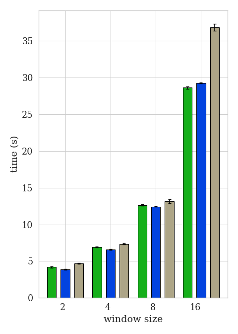
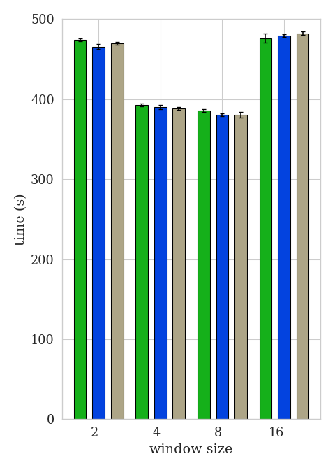
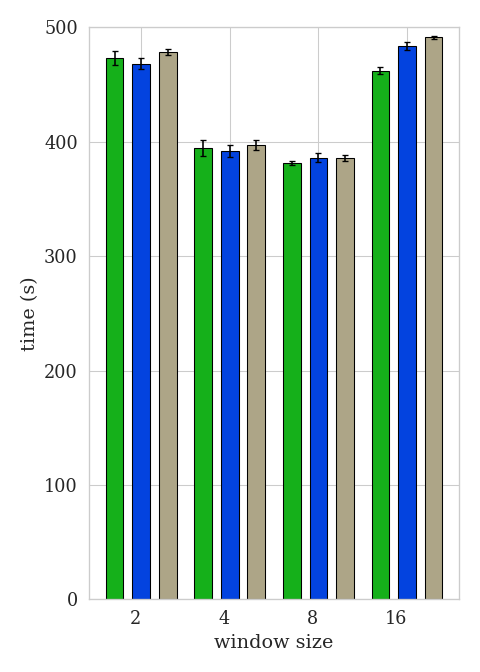
In terms of performance, we find that a naïve approach of using ASP to diagnose time steps does not scale for increasingly large . The performance limitations can be seen in Figure 3: while the total diagnosis time for 8 time steps is just three times that of 2 time steps – and thus scales sublinearly up to this point – diagnosis times for 16 time steps are more than twice as large. For even larger window sizes, e.g., or , performance is worse still, if such window sizes are even feasible – in our experiments, we found to be infeasible and thus used a rolling window for Table 1. A window size of appears optimal from our observations. The overhead of preserving fluents seems negligible.

The rolling window, however, introduces soundness problems to the diagnosis, as information is lost between subsequent invocations of the solver. It is both possible to be too strict and not strict enough about the fluent values to remember. Table 2 shows a few examples of different configurations – varying the window size , the number of time steps considered, and the set of fluents, whose value is carried over to the next window (not including the ab health states, i.e., the previous diagnoses, which are always kept) – leading to different results.
It is well possible, that in the general case, this inconsistency can – or must be – resolved by means of another answer set program and solver call. Particularly, cautious consequences (cf., e.g., [1]) would indicate which fluents must take a certain value in any answer set that assumes a particular diagnosis, but may not be enough to also model which fluents may not ever take a certain value while assuming a particular diagnosis. We leave this gap to future work.
| dataset | params | diagnoses |
|---|---|---|
| stuck | ||
| stuck | ||
| stuck | ||
| stuck | ||
| stuck |
6 Conclusion and Future Work
We demonstrated a diagnosis system based on ASP and FEC and showed how this system can be used to model the temporal behavior of an HVAC system. Our approach enables an explicit modeling of time-dependent phenomena in ASP in the context of MBD. Interestingly, our approach is not only suitable for FDD but also for retrospective analysis. By evaluating a time series after the fact, the system can help identify precisely when a fault began to manifest, offering valuable insights into system dynamics and behavior over time.
We conducted an initial case study on a heating system that demonstrated that the ASP diagnosis model can be used for a practical diagnosis task. While the experiments indicate that a static window approach becomes computationally infeasible very quickly with increasing window sizes, the rolling window variant offers a better trade-off between runtime and window size. However, the rolling window approach comes at the cost of soundness due to information loss between iterations. We showed that maintaining select fluents across solver runs can mitigate this issue to some extent.
In future work, we plan on improving the incremental reasoning and formalizing a more robust preservation strategy for fluents between runs in the case of the rolling window approach. One possibility would be to consider cautious reasoning to infer missing information. Furthermore, we intend to extend our work by considering more case studies from the building domain and other potential application areas, such as diagnosis in the automotive domain.
Another practical challenge worth investigating lies in managing the number of diagnoses returned. Even when only subset minimal diagnoses are considered, we see a rather large number of possible results in the small system studied. Thus, finding strategies for reducing and prioritizing diagnoses is essential in a practical context. For instance, Stern et al. [40] highlight that presenting the full set of diagnoses may be less effective than aggregating them into a health state, which is a compact representation that estimates the likelihood of each component being faulty. It remains to be seen, whether their approach can be meaningfully integrated with ours.
References
- [1] Mario Alviano, Carmine Dodaro, Salvatore Fiorentino, Alessandro Previti, and Francesco Ricca. ASP and subset minimality: Enumeration, cautious reasoning and MUSes. Artificial Intelligence, 320, 2023. doi:10.1016/j.artint.2023.103931.
- [2] Marcello Balduccini and Michael Gelfond. Diagnostic reasoning with A-prolog. Theory and Practice of Logic Programming, 3(4-5):425–461, 2003. doi:10.1017/S1471068403001807.
- [3] Chitta Baral, Sheila McIlraith, and Tran Cao Son. Formulating diagnostic problem solving using an action language with narratives and sensing. In KR, pages 311–322. Citeseer, 2000.
- [4] Moritz Bayerkuhnlein and Diedrich Wolter. Model-based diagnosis with ASP for non-groundable domains. In International Symposium on Foundations of Information and Knowledge Systems, pages 363–380. Springer, 2024. doi:10.1007/978-3-031-56940-1_20.
- [5] Ivan Bratko. Prolog programming for artificial intelligence. Pearson education, 2001.
- [6] Gerhard Brewka, Thomas Eiter, and Mirosław Truszczyński. Answer set programming at a glance. Communications of the ACM, 54(12):92–103, December 2011. doi:10.1145/2043174.2043195.
- [7] Vittorio Brusoni, Luca Console, Paolo Terenziani, and Daniele Theseider Dupré. A spectrum of definitions for temporal model-based diagnosis. Artificial Intelligence, 102(1):39–79, 1998. doi:10.1016/S0004-3702(98)00044-7.
- [8] Zhelun Chen, Zheng O’Neill, Jin Wen, Ojas Pradhan, Tao Yang, Xing Lu, Guanjing Lin, Shohei Miyata, Seungjae Lee, Chou Shen, et al. A review of data-driven fault detection and diagnostics for building HVAC systems. Applied Energy, 339:121030, 2023. doi:10.1016/j.apenergy.2023.121030.
- [9] European Commission. Press release: Commission welcomes political agreement on new rules to boost energy performance of buildings across the EU, December 2023. URL: https://ec.europa.eu/commission/presscorner/detail/de/ip_23_6423.
- [10] German Sustainable Building Council. Wegweiser klimapositiver Gebäudebestand 2022 [Guide to Climate-positive Building Stock 2022]. German Sustainable Building Council, 2022.
- [11] Johan de Kleer and Brian C. Williams. Diagnosing multiple faults. Artificial Intelligence, 32(1):97–130, 1987. doi:10.1016/0004-3702(87)90063-4.
- [12] Thomas Eiter, Giovambattista Ianni, and Thomas Krennwallner. Answer Set Programming: A Primer. Springer, 2009. doi:10.1007/978-3-642-03754-2_2.
- [13] Alexander Feldman, Ingo Pill, Franz Wotawa, Ion Matei, and Johan de Kleer. Efficient model-based diagnosis of sequential circuits. In The Thirty-Fourth AAAI Conference on Artificial Intelligence, AAAI 2020, The Thirty-Second Innovative Applications of Artificial Intelligence Conference, IAAI 2020, The Tenth AAAI Symposium on Educational Advances in Artificial Intelligence, EAAI 2020, New York, NY, USA, February 7-12, 2020, pages 2814–2821. AAAI Press, 2020. doi:10.1609/AAAI.V34I03.5670.
- [14] Gerhard Friedrich and Wolfgang Nejdl. Momo-model-based diagnosis for everybody. In Sixth Conference on Artificial Intelligence for Applications, pages 206–213. IEEE, 1990. doi:10.1109/CAIA.1990.89191.
- [15] Martin Gebser, Amelia Harrison, Roland Kaminski, Vladimir Lifschitz, and Torsten Schaub. Abstract Gringo. Theory and Practice of Logic Programming, 15(4-5):449–463, 2015. doi:10.1017/S1471068415000150.
- [16] Michael Gelfond and Vladimir Lifschitz. The stable model semantics for logic programming. In Robert A. Kowalski and Kenneth A. Bowen, editors, Logic Programming, Proceedings of the Fifth International Conference and Symposium, Seattle, Washington, USA, August 15-19, 1988 (2 Volumes), pages 1070–1080. MIT Press, 1988.
- [17] A Gevorgian, S Pezzutto, S Zambotti, S Croce, U Filippi Oberegger, R Lollini, L Kranzl, and A Muller. European building stock analysis. Eurac Research: Bolzano, Italy, 2021.
- [18] Stephan Gspandl, Ingo Pill, Michael Reip, Gerald Steinbauer, and Alexander Ferrein. Belief management for high-level robot programs. In Toby Walsh, editor, IJCAI 2011, Proceedings of the 22nd International Joint Conference on Artificial Intelligence, Barcelona, Catalonia, Spain, July 16-22, 2011, pages 900–905. IJCAI/AAAI, 2011. doi:10.5591/978-1-57735-516-8/IJCAI11-156.
- [19] Christoph Hutter, Michael Kappert, Ralph Krause, Patrick Müller, André König, Adrian Gebhardt, Falko Ziller, Peter Giesler, and Frank Zeidler. MFGeb - Methoden zur Fehlerkennung im Gebäudebetrieb [MFGeb - methods for fault detection in building operation], 2022. Final Report. URL: https://ibit.fh-erfurt.de/fileadmin/Dokumente/Projekte/IBIT/mfgeb/Abschlussbericht-MFGEB_2022.pdf.
- [20] Ledio Jahaj, Stalin Munoz Gutierrez, Thomas Walter Rosmarin, Franz Wotawa, and Gerald Steinbauer-Wagner. A model-based diagnosis integrated architecture for dependable autonomous robots. In 34th International Workshop on Principles of Diagnosis, 2023.
- [21] Srinivas Katipamula and Michael R Brambley. Methods for fault detection, diagnostics, and prognostics for building systems—a review, part ii. HVAC&R Research, 11(2):169–187, 2005. doi:10.1080/10789669.2005.10391123.
- [22] Roxane Koitz-Hristov and Franz Wotawa. Faster horn diagnosis-a performance comparison of abductive reasoning algorithms. Applied Intelligence, 50(5):1558–1572, 2020. doi:10.1007/S10489-019-01575-5.
- [23] Robert Kowalski and Marek Sergot. A logic-based calculus of events. New Generation Computing, 4(1):67–95, March 1986. doi:10.1007/BF03037383.
- [24] Gerda Langer, Thomas Hirsch, Roman Kern, Theresa Kohl, and Gerald Schweiger. Large language models for fault detection in buildings’ HVAC systems. In Energy Informatics Academy Conference, pages 49–60. Springer, 2024. doi:10.1007/978-3-031-74741-0_4.
- [25] Vladimir Lifschitz. Answer Set Programming. Springer, 2019. doi:10.1007/978-3-030-24658-7.
- [26] Jiefei Ma, Rob Miller, Leora Morgenstern, and Theodore Patkos. An epistemic event calculus for ASP-based reasoning about knowledge of the past, present and future. In Ken Mcmillan, Aart Middeldorp, Geoff Sutcliffe, and Andrei Voronkov, editors, LPAR-19. 19th International Conference on Logic for Programming, Artificial Intelligence and Reasoning, volume 26 of EPiC Series in Computing, pages 75–87, Stellenbosch, South Africa, 2013. EasyChair. doi:10.29007/zswj.
- [27] John McCarthy and Patrick J Hayes. Some philosophical problems from the standpoint of artificial intelligence. Machine Intelligence, 4, 1969. doi:10.1016/B978-0-934613-03-3.50033-7.
- [28] Sheila A McIlraith. Representing actions and state constraints in model-based diagnosis. In Proceedings of the Fourteenth National Conference on Artificial Intelligence and Ninth Conference on Innovative Applications of Artificial Intelligence, AAAI’97/IAAI’97, pages 43–49, 1997. URL: http://www.aaai.org/Library/AAAI/1997/aaai97-007.php.
- [29] Rob Miller and Murray Shanahan. Some alternative formulations of the event calculus. In Antonis C. Kakas and Fariba Sadri, editors, Computational Logic: Logic Programming and Beyond, Essays in Honour of Robert A. Kowalski, Part II, volume 2408 of Lecture Notes in Computer Science, pages 452–490. Springer, 2002. doi:10.1007/3-540-45632-5_17.
- [30] Payam Nejat, Fatemeh Jomehzadeh, Mohammad Mahdi Taheri, Mohammad Gohari, and Muhd Zaimi Abd. Majid. A global review of energy consumption, CO2 emissions and policy in the residential sector (with an overview of the top ten CO2 emitting countries). Renewable and Sustainable Energy Reviews, 43:843–862, 2015. doi:10.1016/j.rser.2014.11.066.
- [31] Ilkka Niemelä. Logic programs with stable model semantics as a constraint programming paradigm. Annals of Mathematics and Artificial Intelligence, 25(3-4):241–273, 1999. doi:10.1023/A:1018930122475.
- [32] Panayiotis M Papadopoulos, Vasso Reppa, Marios M Polycarpou, and Christos G Panayiotou. Distributed diagnosis of actuator and sensor faults in HVAC systems. IFAC-PapersOnLine, 50(1):4209–4215, 2017. doi:10.1016/j.ifacol.2017.08.816.
- [33] Ingo Pill and Thomas Quaritsch. Behavioral diagnosis of LTL specifications at operator level. In Francesca Rossi, editor, IJCAI 2013, Proceedings of the 23rd International Joint Conference on Artificial Intelligence, Beijing, China, August 3-9, 2013, pages 1053–1059. IJCAI/AAAI, 2013. URL: http://www.aaai.org/ocs/index.php/IJCAI/IJCAI13/paper/view/6595.
- [34] Liliana Marie Prikler and Franz Wotawa. Faster diagnosis with answer set programming. In 35th International Conference on Principles of Diagnosis and Resilient Systems (DX 2024), pages 24–1. Schloss Dagstuhl – Leibniz-Zentrum für Informatik, 2024. doi:10.4230/OASIcs.DX.2024.24.
- [35] Gregory Provan. Generating reduced-order diagnosis models for HVAC systems. In Itnl. Workshop on Principles of Diagnosis, Murnau, Germany, 2011.
- [36] Aibing Qiu, Ze Yan, Qiangwei Deng, Jianlan Liu, Liangliang Shang, and Jingsong Wu. Modeling of HVAC systems for fault diagnosis. IEEE Access, 8:146248–146262, 2020. doi:10.1109/ACCESS.2020.3015526.
- [37] Olivier Raiman, Johan de Kleer, Vijay Saraswat, and Mark Shirley. Characterizing non-intermittent faults. In Proceedings of the Ninth National Conference on Artificial Intelligence - Volume 2, AAAI’91, pages 849–854. AAAI Press, 1991. URL: http://www.aaai.org/Library/AAAI/1991/aaai91-132.php.
- [38] Raymond Reiter. A theory of diagnosis from first principles. Artificial Intelligence, 32(1):57–95, 1987. doi:10.1016/0004-3702(87)90062-2.
- [39] Erich Sewe. Automatisierte Fehlererkennung in Heizungsanlagen [Automated Fault Detection in Heating Systems]. PhD thesis, Universität Dresden, 2018.
- [40] Roni Stern, Meir Kalech, Shelly Rogov, and Alexander Feldman. How many diagnoses do we need? Artificial Intelligence, 248:26–45, 2017. doi:10.1016/J.ARTINT.2017.03.002.
- [41] Peter Struss, Raymond Sterling, Jesús Febres, Umbreen Sabir, and Marcus M. Keane. Combining engineering and qualitative models to fault diagnosis in air handling units. In Proceedings of the Twenty-First European Conference on Artificial Intelligence, ECAI’14, pages 1185–1190. IOS Press, NLD, 2014. doi:10.3233/978-1-61499-419-0-1185.
- [42] Michael Thielscher. A theory of dynamic diagnosis. electronic transactions on artificial intelligence. Electron. Trans. Artif. Intell., 1:73–104, 1997. URL: http://www.ep.liu.se/ej/etai/1997/004/.
- [43] Michael Thielscher. Introduction to the fluent calculus. Electron. Trans. Artif. Intell., 2:179–192, 1998. URL: http://www.ep.liu.se/ej/etai/1998/006/.
- [44] Balaje T. Thumati, Miles A. Feinstein, James W. Fonda, Alfred Turnbull, Fay J. Weaver, Mark E. Calkins, and S. Jagannathan. An online model-based fault diagnosis scheme for HVAC systems. In 2011 IEEE International Conference on Control Applications (CCA), pages 70–75, 2011. doi:10.1109/CCA.2011.6044486.
- [45] Christoffer Thuve and Hema Pushphika Yuvraj. Life cycle assessment of a combustion engine-mapping the environmental impacts and exploring circular economy. Master’s thesis, Chalmers University of Technology, 2022.
- [46] Louise Travé-Massuyès and Teresa Escobet. Bridge: Matching model-based diagnosis from FDI and DX perspectives. Fault Diagnosis of Dynamic Systems: Quantitative and Qualitative Approaches, pages 153–175, 2019. doi:10.1007/978-3-030-17728-7_7.
- [47] Franz Wotawa. On the use of answer set programming for model-based diagnosis. In Hamido Fujita, Philippe Fournier-Viger, Moonis Ali, and Jun Sasaki, editors, Trends in Artificial Intelligence Theory and Applications. Artificial Intelligence Practices - 33rd International Conference on Industrial, Engineering and Other Applications of Applied Intelligent Systems, IEA/AIE 2020, Kitakyushu, Japan, September 22-25, 2020, Proceedings, volume 12144 of Lecture Notes in Computer Science, pages 518–529. Springer, 2020. doi:10.1007/978-3-030-55789-8_45.
- [48] Franz Wotawa and David Kaufmann. Model-based reasoning using answer set programming. Appl. Intell., 52(15):16993–17011, 2022. doi:10.1007/S10489-022-03272-2.