Automating Control System Design: Using Language Models for Expert Knowledge in Decentralized Controller Auto-Tuning

Abstract
Fully-automated optimal controller design for engineering systems is a challenging task. While, optimization-based, automated control parameter tuning techniques have been widely discussed in the literature, most works do not discuss expert knowledge requirements for system design, which result in significant human intervention. In this work, we discuss a multistage controller tuning framework for decentralized control that highlights expert knowledge requirements in automated controller design. We propose a methodology to automate the input-output pairing and stage definition steps in the framework using Large Language Models (LLMs) for a family of multi-tank benchmarks. We achieve this by proposing a mathematical language to describe the system and design an algorithm to bind this mathematical representation to the input prompt space of an LLM. We demonstrate that our methodology can produce consistent expert knowledge outputs from the LLM with over 97% accuracy for the multi-tank benchmarks. We also empirically show that, correct stage definition by the LLM can improve tuned controller performance by up to 52%.
Keywords and phrases:
controller auto-tuning, automated system design, large language modelsCopyright and License:
![[Uncaptioned image]](x1.png) © Marlon J. Ares-Milian, Gregory Provan, and Marcos Quinones-Grueiro; licensed under Creative Commons License CC-BY 4.0
© Marlon J. Ares-Milian, Gregory Provan, and Marcos Quinones-Grueiro; licensed under Creative Commons License CC-BY 4.0
2012 ACM Subject Classification:
Computing methodologies Knowledge representation and reasoningSupplementary Material:
Software (Source Code): https://github.com/mjares/DX2025_LLMs_ExpertKnowledge.gitarchived at
 swh:1:dir:81a0af39fd36f5d0fe1daae775b1e460067fd364
Funding:
This work was supported by Science Foundation Ireland under Grant 13/RC/2094.Editors:
Marcos Quinones-Grueiro, Gautam Biswas, and Ingo PillSeries and Publisher:
 Open Access Series in Informatics, Schloss Dagstuhl – Leibniz-Zentrum für Informatik
1 Introduction
Most modern engineering issues are framed as systems. For example, vehicles, robots, and industrial machines are all systems, albeit different, and each have sub-systems and components that work in close relation to achieve their intended functions. The development of modern engineering systems goes through three main stages: design, production, and operation. Proper design is the focus of this paper, since it enables engineering systems to meet desired performance objectives, e.g.: development and operational costs, safe operation, and robustness, while also supporting validation and verification, enhancing the production and operation stages [8]. However, optimal system design is a very challenging task due to the extensive space of system configurations, components, and parameters [18] that must be explored. In spite of all the advances in automation to date, solving the design problem often requires significant human expertise and iterative design protocols [7]. Therefore, a strong motivation exists to develop automated optimal design methodologies that meet desired objectives while reducing the tedious, time-consuming, and costly aspects of manual design.
With the development of cyber-physical systems and the internet of things, automation has become ubiquitous in modern engineering systems [8] and the key component for automation in any modern system is the controller. A controller (or control algorithm) refers to the sub-system that receives information from real or estimated measurements and operates the actuators in order to regulate system variables with different objectives. The design of controllers for engineering is a complex task, consisting of multiple components and steps. Controllers are usually defined by parametric functions, which results in a problem well-known as controller tuning: the design step where controller parameters are adjusted (or tuned) to meet desired performance objectives. Traditional controller tuning is done manually, requiring an iterative design process based on expert knowledge. This is an inefficient approach that usually results in sub-optimal solutions, which has motivated significant research on automated design of controller parameters, known as controller auto-tuning.
Many modern controller auto-tuning solutions resort to an iterative optimization approach in which some performance objectives are evaluated (either in simulation or hardware) and the controller parameter space is explored using some optimization algorithm until the best set of parameters is obtained; this is done through some combination of system-model knowledge, expert knowledge, and historical data, and includes tools like reinforcement learning [13], evolutionary optimization [16], and Bayesian optimization [17]. Even though the controller parameter search itself has been widely automated, the controller design problem (including controller parameter design) still requires abundant expert knowledge in different steps of the process that are often ignored in the associated literature [2]. Some of the open challenges in fully automated controller design include aspects of the parameter optimization problem definition like defining constraints, defining and restricting the search space, and defining the cost function, as well as other aspects of the control system design such as control loop definition (also known as input-output pairing) [12]; all of these are currently solved, in the majority of cases, using expert knowledge. In this work, we propose a methodology to automate expert knowledge for a subset of steps in the control system design problem: input-output (I/O) pairing and stage definition for a multistage controller auto-tuning framework. We use Large Language Models (LLMs) to meet these expert knowledge requirements.
LLMs are deep learning models trained over a large volume of natural language data spanning multiple topics and scientific disciplines while following task-agnostic architectures [5]. Therefore, they are often used as a form of zero-shot or few-shot transferable models with a variety of applications [14][7][19]. This makes LLMs a prime target for automating expert knowledge, a task that is often unstructured and heavily relies on natural language interactions. While LLMs have shown positive results, multiple challenges persist in terms of LLM output formatting, consistency, and accuracy, generalization to more complex topics/benchmarks, factually incorrect responses, etc. Therefore, multiple works have focused on how to maximize performance from an already trained LLM, with prompt engineering (PE) being the most discussed approach. PE is based on the fact that a well-designed (natural language) prompt can dramatically improve the quality of the output in an LLM [10]. In this paper, we discuss a PE methodology to automate expert knowledge in control system design.
The contributions of this work are as follows: (1) We highlight existing challenges in automated controller design and automate expert knowledge using LLMs. We focus on expert knowledge requirements for I/O pairing and stage definition in a multistage decentralized controller auto-tuning framework. (2) We define a mathematical language based on system topology to describe a family of industrial multi-tank benchmarks. (3) We propose a system-informed prompt engineering algorithm to bind the mathematical language to the input prompt space of an LLM in order to automate expert knowledge for controller design. (4) We empirically evaluate the effectiveness of LLMs for substituting expert knowledge in I/O pairing and stage definition tasks for a family of multi-tank benchmarks using performance metrics like: proper formatting of output prompt and correct expert knowledge provided. We show that the LLM can produce expert knowledge recommendations with over 97% accuracy with consistent formatting for I/O pairing and stage definition. (5) We empirically evaluate, for the first time (to the best of our knowledge), the relevance of controller tuning order on performance of tuned controllers, when tuning decentralized controllers independently and sequentially, for a family of multi-tank benchmarks. We show that, depending on the complexity of the system, and the degree of coupling between its components, a correct stage definition can improve the tuned controller performance by up to 52%
2 Related Work
2.1 Automated Controller Design
When discussing automated controller design, most works focus on controller auto-tuning, which is popularly framed as a derivative-free optimization problem [16][17]. While gradient-based methods are also used for controller auto-tuning [13], derivative-free formulations have the desired advantage of making little or no assumptions on objective or constraint functions.
Multiple authors have proposed metaheuristic approaches to controller auto-tuning, with [16] doing a detailed survey on evolutionary optimization algorithms for multiple-input-multiple-output processes. However, Bayesian optimization (BO) approaches have become quite popular in recent years, due to their high sample efficiency [2] and overall performance. For example [17] present a joint tuning methodology that uses BO to simultaneously tune an LQR controller, an unscented Kalman Filter (UKF), and a guidance and navigation system for an autonomous underwater vehicle (UUV), yielding satisfactory results across multiple objectives. Most of the available solutions focus strictly on the parameter search itself and how to solve it using some optimization tool, leaving the design of the optimization problem, or the control algorithm, as an expert knowledge requirement.
In their work, [2] also propose a Bayesian optimization solution for controller auto-tuning of PID controllers in an underwater vehicle, improving the computational complexity of the controller tuning task by decomposing the search space into smaller dimension subspaces. In order to do so, they propose a multistage framework that aims to formalize all the necessary steps in automated controller design. This formalization highlights a variety of existing challenges in automated controller design that are often ignored, or underexplored in recent works. Examples of these challenges are how to define the parameter search space, the constraints, or the cost function for the optimization problem, issues that are often not discussed, or attributed to expert knowledge. Similarly, how to define the stages in the multistage framework defined in [2] is still one of the open problems highlighted in the paper.
An attempt to address one of these expert knowledge requirements can be found in [12], where an optimal control formulation is proposed in order to simultaneously optimize the controller parameters and produce an I/O pairing for the system. I/O pairing, or control loop design, is often assumed to be already defined in most controller auto-tuning works [17], when, in reality, it is usually performed through expert knowledge.
Overall, state-of-the-art research on automated controller design is significantly challenged by expert knowledge requirements across different stages of the problem.
2.2 LLMs in System Design
Several papers have used LLMs for some aspect of system design, but fundamentally most approaches still adopt significant manual modeling, employing LLMs after the design process.
[14] uses a five-step LLM-based prompting approach that requires as inputs a piping and instrumentation diagram (P&ID) and natural language prompts. They evaluate the approach on a one-tank, one three-tank, and one four-tank system. Our approach differs in that we focus on control tuning and not diagnostics, we use a formal language for LLM prompting that provides guarantees about optimality of controller design, and we focus on control-model optimization and not just model generation.
A closely related approach, SmartControl [19], automatically determines the most suitable PID parameters to achieve the specified performance targets using PSO and DE algorithms. This process includes selecting the optimal gains that will ensure the system’s fast and stable response. After optimization, the closed-loop step response is simulated and basic performance metrics (such as settling time, rise time, overshoot, etc.) are calculated and presented to the user via an interactive graphical interface. SmartControl emphasizes interactive design, allowing users to engage directly with the LLM agent to refine the controller design. The approach in the provided paper is more automated; the LLM generates the I/O pairing and stage definitions without direct user interaction during that phase.
ControlAgent [7] employs a range of techniques for integrating domain knowledge, e.g., a knowledge graph or other structured representation of control engineering principles. Our approach aims for full automation once the initial system description is provided; in contrast, ControlAgent involves more interactive elements, allowing users to refine the design process through feedback or iterative refinement with the LLM.
2.3 Systems Modeling using Component-Based Languages
Several frameworks exist to define systems based on interconnected component models, e.g., bond graphs, Simulink, and Modelica. The proposed approach is a fundamentally different framework from such approaches, most of which rely on manually-defined component models.
The approach is most similar to bond graphs (which focuses on representing energy flow and causality), although the current usage is quite different. In a bond graph, nodes consist of a standardized set of elements (e.g., C for capacitance, I for inertia, etc.) and edges/junctions represent system components and their interactions. The resulting graph allows for deriving system equations and performing simulations. Our proposed graph model is simpler than a bond graph model, as it does not specify the inherent physical properties of the nodes.
The two approaches are not mutually exclusive. One could conceivably use bond graphs to model a multi-tank system and then use the resulting model (or a simplified representation of it) as input to the LLM-based system for automated control design. The bond graph would provide a structured representation of the system’s dynamics, while the LLM would handle the more complex task of selecting appropriate control strategies and parameters. The paper, however, focuses solely on the LLM-based approach without explicit integration of bond graphs. The paper’s graph representation is a simplified topological representation, not a full bond graph model.
3 Preliminaries
3.1 Decentralized parametric control
Let’s define a controller by a tuple where is the space of system measurements/outputs (e.g.: level in a tank, altitude in a drone), is the space of system inputs (e.g. liquid flow from a pump, propeller commands in a quadcopter), and is a control algorithm that produces a system input at every timestamp considering system inputs and outputs from previous system interactions. We are interested in a family of control frameworks called decentralized parametric controllers, which are commonly used in industrial and robotic systems [2].
A parametric control algorithm is a parametric function such that , with , where the control algorithm is defined by a set of parameters that must be previously adjusted (tuned). Parametric controllers are very common, with the proportional-integral-derivative controller and its P, I, and D parameters being the industry standard [16].
A decentralized control approach is defined by a set of independent control algorithms where every control algorithm matches a single system input with a single system output , and the changes in that system input are only conditioned by the corresponding system output, i.e.: . This is a common simplification in control system design [2] with assumptions regarding system coupling. The implications of these assumptions are discussed further in this paper.
3.2 Directed graphs
A graph is defined by a tuple where is a set of elements called vertices and is a set of pairs called edges [6]. An edge describes a relationship between two vertices, we can say that an edge joins two vertices. For the purpose of this work, we are interested in graphs with the following properties:
-
Directed: In a directed graph, the edges are ordered pairs and have an implied direction, i.e.: . An edge in a directed graph is called a directed edge.
-
Simple: A simple graph is a graph without loops. A loop in a graph is defined as an edge that joins a vertex to itself, i.e.: .
-
Edge-Labeled: In an edge-labeled graph , a labeling function is defined to assign a label from the label set to each edge in the edge set.
Let’s discuss some graph theory concepts that will be relevant in the rest of this work [4].
Definition 1 (Directed Path).
A directed path is a sequence of distinct edges in a graph that joins a sequence of distinct vertices such that is a directed edge.
Definition 2 (Strongly Connected Component).
A directed graph is considered to be strongly connected if every vertex is reachable from every other vertex in the graph, i.e.: for any vertex pair , there is at least one directed path that goes from to . A strongly connected component of a graph is a subgraph that is strongly connected, and is maximal with this property, i.e.: no additional edges or vertices from can be included in without breaking its property of being strongly connected.
Strongly connected components in a graph can be computed in linear time by a variety of algorithms (e.g.: depth-first-search algorithms) [4].
3.3 Large Language Models
Let us define the prompt space [11]. The elements in are a composition of tokens selected from a token vocabulary , where can be a sequence of tokens of any length . An LLM is then defined as a transformation where, for a given input prompt , the model produces an output prompt .
A common feature in LLM APIs is the system prompt. A system prompt permeates every interaction [20] with the LLM, providing context, setting the role and the tone for the LLM responses, ensuring output prompt formatting, etc. Particular implementations of the system prompt vary depending on the LLM; in some cases it is provided as an initial prompt before the input prompt [11], while in other cases a dedicated system token is implemented. For the purpose of this work, we are interested in LLMs with system prompt () options, i.e.: . In Section 4.4, we define bindings from a graph language describing a family of physical systems to the input and system prompt spaces.
3.4 Bayesian optimization
Bayesian optimization is a technique for globally optimizing black-box functions that are expensive to evaluate [9]. We consider the global minimization problem: with input space and objective function . We consider costly-to-evaluate functions for which we have a limited number of evaluations available before we propose an optimum in at most iterations. We assume we have access only to noisy evaluations of the objective , where is i.i.d. Gaussian noise with variance . Finally, we make no assumptions regarding gradients or convexity properties of .
The main steps of a BO routine in iteration involve (1) response surface learning, (2) optimal input selection , and (3) evaluation of the objective function at .
The BO framework uses the predictive mean and variance of a Gaussian Process (GP) [15] model to formulate an acquisition function that trades off exploitation, testing promising controller parameters given the current knowledge, with exploration, sampling unexplored regions of the design space. The BO algorithm can be initiated without any past observations, but it is usually more efficient to calibrate the GP model hyper-parameters and calculate a prior by first collecting an initial set of observations.
4 Methodology
4.1 Controller tuning framework
We define the controller tuning task as a multi-objective optimization (MOO) problem:
| (1) |
where are controller parameters and are objectives. We consider an MOO problem for a more general definition; however, controller auto-tuning is commonly framed as a scalar objective optimization problem. Our proposed framework is fully compatible with both the multi-objective and scalar-objective definitions of the problem. We assume a system with decentralized parametric controllers; other than that, the proposed framework makes no assumptions on the parameter and objective spaces. This general tuning problem can be redefined as a multistage optimization problem where a subset of controllers is tuned at every stage. Each stage can be defined as an MOO sub-task. Fig. 1 illustrates the process.
At stage of the tuning process, a subset of control parameters () are tuned to minimize some stage-specific objectives (), given reference signal . The rest of the control parameters are fixed at a previous stage, or before the tuning process begins, through the constraint parameters . At each stage, a subset () of the optimal control parameters () is produced as a result of an MOO sub-task described below.
The I/O pairing and the definition of the stages are task-specific steps, both of which are commonly solved using expert knowledge [2][16]. The main contribution of this work is a methodology to automate this expert knowledge requirement and produce an I/O pairing and stage definition using LLMs. Further details on these steps can be found in Section 4.3.

The controller tuning optimization task is decomposed into sub-tasks defined as:
| (2a) | ||||
| s.t. | (2b) | |||
| (2c) | ||||
where (2c) is a constraint that sets control parameters to specified values () from a previous stage or from before the tuning process begins.
These optimization sub-tasks can be solved using any optimization algorithm, as long as the cost function and search space are properly defined. For the purpose of this work, we use Bayesian Optimization to solve the optimization sub-tasks; we refer the reader to [2] for a more detailed discussion on the optimization sub-tasks and the use of Bayesian Optimization.
4.2 Graph Language For System Representation
We now define a language, in the form of an enhanced system graph, to describe physical systems in terms of reservoirs, actuators, and connections:
Definition 3 (Enhanced System Graph).
An enhanced system graph is a directed, simple (no loops), edge-labeled graph that describes relationships between tanks and pumps in a multi-tank system. The graph is separated into two subgraphs where is the actuator subgraph and is the tank subgraph.
Let’s first discuss the tank subgraph which describes relations between the different tanks. Each vertex in the set , represents a tank in the system, where tank labels (vertices) are assigned arbitrarily, and is the number of tanks in the system. The edge set represents a liquid flow connection between the tanks. The direction of the edges represents possible flow directions. A regular directed edge represents liquid flow that is only feasible from tank to tank , for example, the drain of a gravity-drained tank that feeds a tank below it. A bidirectional edge represents an interconnection between tanks where liquid flow can occur in both directions, for example, two horizontally aligned tanks connected by a pipe.
Based on the edge directionality and the semantics of edges, we can assign a labeling to edges for constructing LLM prompts. The edge-label set provides the necessary information about the relationships between the tanks for prompt engineering. The labeling function is defined for any edge :
| (3) |
where an edge is labeled if it is bidirectional (i.e.: the opposite direction edge is also in the graph) and or if the edge is not bidirectional (i.e.: the opposite direction edge is not in the graph). An edge is labeled if vertex is of lower numerical value than vertex and if the opposite is true. Note that the value of the vertices, which effectively act as labels for the tanks, are assigned arbitrarily, and the purpose of this labeling strategy is to ensure a consistent distinction between types of edges, which becomes relevant when building natural language prompts for the LLM. Therefore, the distinction between and edges is done without loss of generality.
We then define the actuator subgraph where each vertex in represents an actuator in the multi-tank system, e.g.: a pump. Every edge in represents a connection between an actuator and a tank, where an edge is always directed from an actuator vertex to a tank vertex. One actuator vertex can be connected to multiple tank vertices. The labeling function for the actuator subgraph maps each actuator vertex to a corresponding vertex label that describes attributes of the fluid going through the actuator which may include: temperature of the fluid, composition or concentration of the fluid, etc.; e.g.: .
Fig. 2(a) shows an example three-tank system and its corresponding graph representation (Fig. 2(b)). Elements from the tank subgraph are presented in continuous lines while the actuator subgraph is represented by discontinuous lines.


4.3 Input Output Pairing and Stage Definition
In this section we formalize the concepts of I/O pairing and stage definition, and how they relate to the controller auto-tuning framework defined in Section 4.1.
4.3.1 Input-Output Pairing
Let us consider a system with input space consisting of system inputs, corresponding to the output of decentralized controllers. Let us also consider an output space consisting of outputs, corresponding to known system variables (either by direct measurement or estimation). In the context of decentralized controllers, we define an I/O pairing as a matrix where if input and output are paired, and otherwise. In practice, an input and an output being paired means that the value of the output is used to compute the paired system input through the respective control algorithm. Every input must be paired with an output exactly once.
Let us illustrate this concept using the example from Fig. 2. This three tank system is fed by three input pumps, pump 1 feeds tank one with an input flow , pump 2 feeds tank two with an input flow , and pump 3 feeds tank three with an input flow . The levels in the three tanks are measured, resulting in the respective outputs , , and . The I/O pairing task in this case is trivial, since it is obvious we want to control the level in tank using the pump that feeds tank . Assuming a set of inputs: {FlowPump1, FlowPump2, FlowPump3}, respectively , and a set of outputs: {LevelTank1, LevelTank2, LevelTank3}, respectively ; Fig. 3 shows example I/O pairings for the system.
I/O pairing is equivalent in the literature to control loop design [12] since, pairing an input and an output defines a feedback loop for the corresponding controller. Following the correct input-output pairing (Fig. 3(a)), we define three control loops: {FlowPump1-LevelTank1, FlowPump2-LevelTank2, FlowPump3-LevelTank3}. We formalize a control loop as a tuple and tuning a control loop refers to tuning the corresponding controller.
4.3.2 Stage Definition
Once we determine an I/O pairing in the system, we must define the stages for the multistage optimization problem presented in Section 4.1. This involves defining the total number of stages and, for every stage , the controller tuned at this stage and the control parameters fixed from previous stages. This information is then summarized into the stage-specific parameters for each optimization subtask (2). In order to produce a concise description of the stages in the framework, we define a stage matrix where every row represents a stage, and every column represents a control loop. An element in the matrix is if the controller for control loop is tuned at stage , if control loop is open at stage , and if control loop is closed at stage using control parameters tuned in a previous stage. For the purpose of this work, every controller must be tuned exactly once, and at least one controller must be tuned at every stage.
What is a correct stage definition, as well as the relevance of this process, is task-specific, and is often determined from expert knowledge based on the couplings (I/O interactions) in the system. Ideally, the output of a control loop should only be affected by the corresponding input . However, this is often not the case and output is affected by variations in the inputs of other loops ; when this happens, we say loop is coupled with loop . This relationship is not symmetric, if control loop is coupled with control loop , control loop can be decoupled from , where variations in input do not affect output . In the context of controller tuning, we tune control loops that are isolated (i.e.: not coupled to any loops) first and then tune the coupled loops. When tuning a controller for a coupled loop , if possible, we want all the loops that is coupled with to be closed using control parameters tuned in previous stages, which minimizes variations in the variables from the coupled loops, making behave like a decoupled loop. Following this methodology we can see that correct stage definition for a system is not always unique.
Let us illustrate the concept of stage definition using the example from Fig. 2. The control loops in the system are (Section 4.3.1): {FlowPump1-LevelTank1, FlowPump2-LevelTank2, FlowPump3-LevelTank3}, for simplicity, . In this case, the correct stage definition should start by tuning the control loop corresponding to tank 1 . This is an isolated loop in the system since, due to the connection between tank 1 and 3 being gravity-based, no variations in the pumps feeding tank 2 and 3 can affect the level in 1, while variations in the pump feeding tank 1 can affect the level in tanks 2 and 3. Tanks 2 and 3 are interconnected and flow between them can go in either direction, making loops and coupled both ways; therefore, these loops can be tuned in any order. In summary, any stage definition that tunes control loop in the first stage, and maintains this loop closed for further stages, is considered correct. Fig. 4 shows an example of a correct and incorrect stage definitions of the system, replacing with .
4.4 LLM prompt design
In this section we discuss how to design input and system prompts (Section 3.3) for an LLM in order to automate I/O pairing and stage definition, given limited structural knowledge of the system, for a family of multi-tank systems. We present an algorithm for input prompt design given the graph representation of the system defined in Section 4.2.
4.4.1 Input prompt design
In this section we describe the methodology (Algorithm 1) used to design an input prompt for stage definition in a multi-tank system assuming a graph representation (Def. 3) of the system is available. The resulting input prompt consists of 6 distinct sections: introduction, hierarchical relations, interconnections, actuators, input-output-loop list, and task instruction.
We start by introducing the system and the number of tanks () in it and then describe the hierarchical relations between tanks. In order to do this, we define a set of single direction edges, . Every edge in represents a hierarchical relation between tanks where only one flow direction is feasible, whether it is due to gravity or a pump forcing a fixed flow. This section of the prompt design algorithm generates a sequence of sentences (one for each element in ) that describe the hierarchical relations between pairs of tanks using the corresponding labels . The set is ordered from lowest to highest according to ( is the minimum between and ). The edge ordering of set is done for consistency, which we have found to impact performance significantly when designing the prompt.
We then describe groups of tanks that are interconnected. To do so, we define a set of subgraphs . For every connected subgraph , we produce a sentence highlighting interconnection between the tanks represented by the subgraph. The tanks don’t need to be horizontally aligned, we use this sentence structure to stay consistent with the vertical alignment description of the system hierarchy.
Afterwards, we describe the actuators in the system and their relationship with the corresponding tanks. For the purpose of this work, we only consider the family of systems with actuators as pumps, however, the actuator space can be easily expanded by making the actuator label space more expressive. First we list the number of pumps . Then, we add a sentence to the prompt for each actuator , where we list the set of tanks that are fed by pump . If the fluid through the actuator has associated attributes, these are added to each actuator sentence by means of .
Subsequently, we provide an ordered list of inputs and outputs in the system and, for the case of the stage definition task, we also provide a description of the control loops. Finally, instructions about the task (stage definition or I/O pairing) are provided. Fig. 5 shows the resulting input prompt for stage definition designed for the example system in Fig. 2.
A system with three gravity drained tanks filled with fluid. Tank 1 is positioned above tank 3 and the drain of tank 1 feeds tank 3 as an input flow. Tank 2 and tank 3 are horizontally aligned and interconnected by a pipe. The system is fed by 3 pumps, producing input flows. Pump 1 feeds tank 1. Pump 2 feeds tank 2. Pump 3 feeds tank 3.
Inputs: [FlowPump1, FlowPump2, FlowPump3]
Outputs: [LevelTank1, LevelTank2, LevelTank3]
3 control loops with 3 PID controllers:
[FlowPump1-LevelTank1, FlowPump2-LevelTank2, FlowPump3-LevelTank3]
Propose a methodology to tune the controllers sequentially
4.4.2 System Prompt Design
A well-designed system prompt can enhance the performance of the LLM interaction. The system prompt design strategy consists of four sections: a role statement, a description of the task, output formatting instructions, and an output format example.
The role statement is a common practice in system prompt design, usually implemented with a single sentence in the form: “You are {role}”. In this case we define the role as “expert control engineer”. We then describe the desired task (I/O pairing or stage definition).
The large output prompt space , along with the stochastic nature of the LLM (assuming non-zero temperature), results in challenges when processing the LLM output programmatically in a fully automated framework. For example, in the case of I/O pairing, we want to produce a matrix like the one in Fig. 3 from a natural language output . To parse this output correctly, a consistent output prompt formatting is desired. We ensure this by adding formatting instructions to the system prompt, as well as an example desired output.
System prompts are independent from the particular configuration of the multi-tank system, and their design depends on the desired task. Figures 6(a) and 6(b) show the system prompts used for the I/O pairing and stage definition tasks respectively.
You are an expert control engineer. Provide a matrix showing recommended input-output pairings for a system. Your answer must contain a table wrapped in <ans></ans> and nothing more. The table must be formatted exactly as described below:
- Columns: System Outputs
- Rows: System Inputs
- Cells: “1”=input and output are paired, “0”=input and output are not paired
All inputs must be paired exactly once.
Example:
<ans>
[Output1] [Output2] [Output3] … [OutputN]
Input1 0 1 0 … 0
Input2 1 0 0 … 0
…
InputS 0 0 1 … 0
</ans>
You are an expert control engineer. Your task is to provide a matrix showing sequential PID controller tuning order. Upstream control loops should be tuned first. Your answer must contain a table wrapped in <ans></ans> and nothing more. The table must be formatted exactly as described below:
- Columns: PID controllers by control loop
- Rows: Tuning steps
- Cells: “1”=tuned at this step, “0”=opened at this step, “2”=tuned in previous step
At least one controller must be tuned per step. Each controller is tuned exactly once. Example:
<ans>
[Loop1] [Loop2] [Loop3] … [LoopN]
Step1 0 1 0 … 0
Step2 1 2 0 … 0
…
StepS 0 2 1 … 2
</ans>
5 Experimental Design
5.1 Performance Metrics
In order to evaluate the proposed I/O pairing and stage definition methodologies we use multiple performance metrics which evaluate output prompt formatting and accuracy, as well as auto-tuned controller performance.
5.1.1 Performance Metrics for LLM output
Consider a system benchmark , e.g.: three cascading tanks, two interconnected tanks, and a task . Let’s then assume an LLM is prompted with the corresponding system () and input () prompts such that the output prompt is produced. Let us define the following set of performance metrics in order to evaluate output prompt : correct formatting, accuracy, and percentage of accurate over correctly formatted.
Correct Formatting.
For a given task and benchmark , let us define a correctly formatted set with all the output prompts that match the restrictions imposed in the corresponding system and input prompts . An output prompt is considered correctly formatted if . We are also interested in the average performance over a set of interactions (to account for the stochastic nature of the LLM). We define percent of correctly formatted outputs as:
| (4) |
Accuracy.
For a given task and benchmark , let us define a ground truth set with all the output prompts that an expert would consider correct. An output prompt is considered accurate if it is in the ground truth set . An output prompt must be correctly formatted in order to be accurate, i.e.: . Similarly to proper formatting, we are interested in the percent of accurate outputs:
| (5) |
Accuracy over Correct Formatting.
Finally, we define a metric for LLM outputs that is only valid over multiple interactions with the LLM: . The purpose of this metric is to evaluate the ability of the LLM to produce accurate outputs, assuming that this output is correct (hence ignoring incorrectly formatted responses). This is arguably the most important metric for LLM outputs due to the fact that, if an output is incorrectly formatted, the interaction with the LLM can be repeated until a correctly formatted output is produced. This approach is viable since expert knowledge is not required to verify the output formatting, however, a low correct formatting metric can lead to higher inference costs due to unnecessary interactions.
5.1.2 Performance of tuned controllers
We are also interested in evaluating the performance of the tuned controllers given a stage definition produced by the LLM. This performance metric is only valid for properly formatted output prompts (). We are particularly interested in evaluating performance of tuned controllers for different stage definitions in order to validate our hypotheses that stage definition is critical to achieve good controller performance when auto-tuning decentralized controllers sequentially, which, to the best of our knowledge, is a comparison that has not been performed before. We do not evaluate the performance of the tuned controllers for different I/O pairings since this is a well-known topic in the literature [12].
We measure performance of tuned controllers using the integral absolute error (IAE) metric [16][12][2], a well known controller performance metric that evaluates the ability of the system, using the tuned controllers, to minimize the error in the measured variables with respect to a reference trajectory . We use MATLAB bayesopt method to implement a Bayesian optimization algorithm (with IAE as the cost function) and solve the controller tuning problem described in Section 4.1 for different stage definitions proposed by the LLM interactions. A detailed explanation of the full auto-tuning algorithm can be found in [2].
5.2 Multi-tank benchmarks
In this section, we will describe the different multi-tank configurations used to empirically evaluate the proposed methodology. In order to highlight the details of each task, we use three distinct set of benchmarks to evaluate: I/O pairing LLM output, stage definition LLM output, and performance of tuned controllers for stage definition.
For I/O pairing evaluation we use 5 configurations of the multi-tank system which include: (1) three cascaded tanks (Fig. 8(a)) and (2) four cascaded tanks (Fig. 8(c)). We also evaluate I/O pairing on three system configurations taken from [12], where input-output pairing is framed as an optimization problem, and solved iteratively. These configurations are: (3) a well-known quadruple tank system (Fig. 9(a)), (4) a variation of the quadruple tank system (Fig. 9(b)), and (5) a single tank system where both level and temperature in the tank are controlled (Fig. 9(c)). Table 1 shows the list of configurations for I/O pairing evaluation.
For stage definition LLM output evaluation we use 7 configurations of the multi-tank system: (1) two cascaded tanks (Fig. 7(a)), (2) alternative two cascaded tanks (Fig. 7(b)), (3) two interconnected tanks (Fig. 7(c)), (4) three cascaded tanks (Fig. 8(a)) (5) alternative three cascaded tanks (Fig. 8(b)), (6) the three tank system illustrated in Fig. 2, and (7) four cascaded tanks (Fig. 8(c)). Table 2 shows the list of configurations for stage definition LLM output evaluation. The pairs of configurations (1)-(2) and (4)-(5) respectively describe a system with the same layout, but different tank labeling. We evaluate alternative labeling of the same configurations to test robustness of the prompt design methodology to small changes in the system description, which has shown to be a challenging task [3].

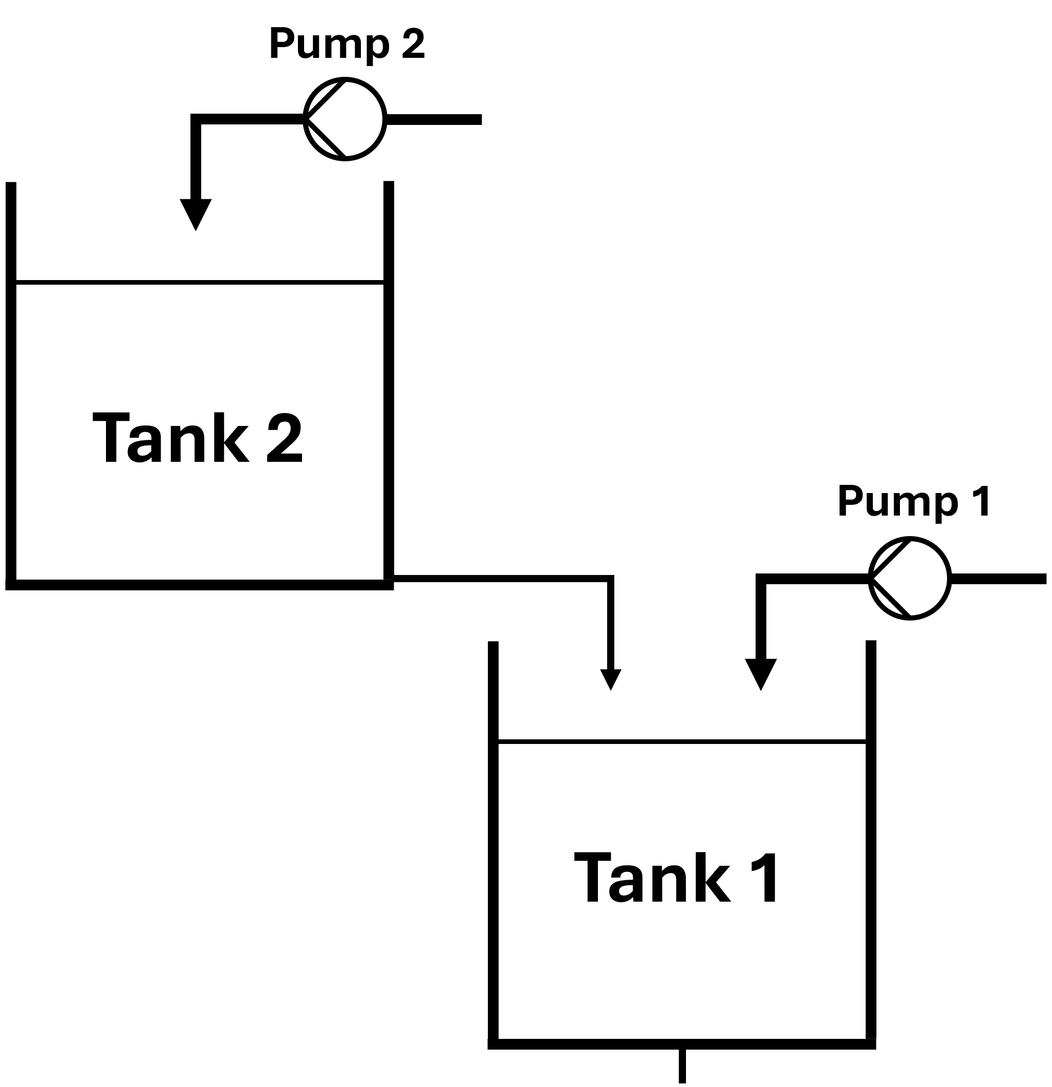
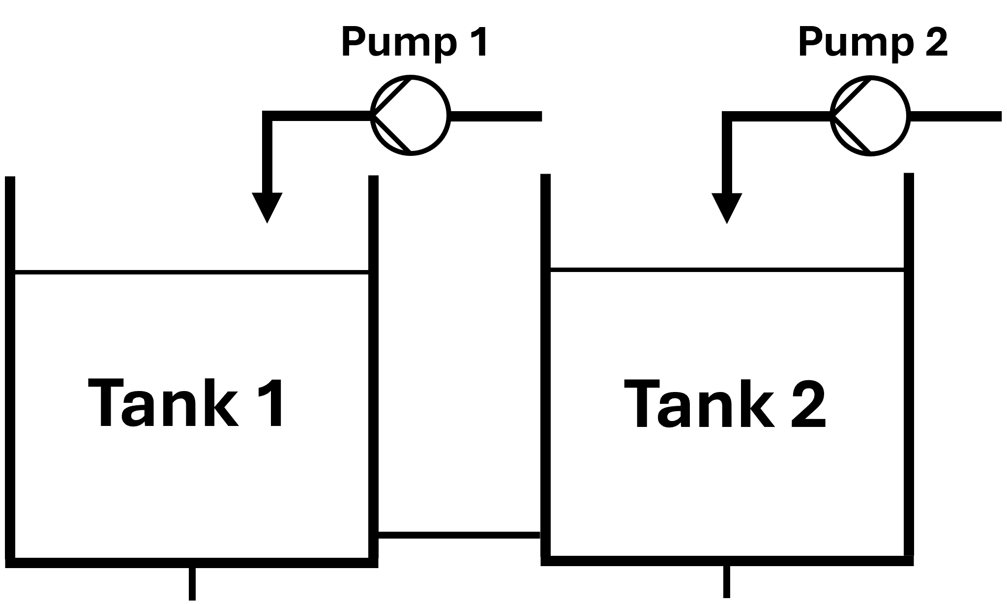
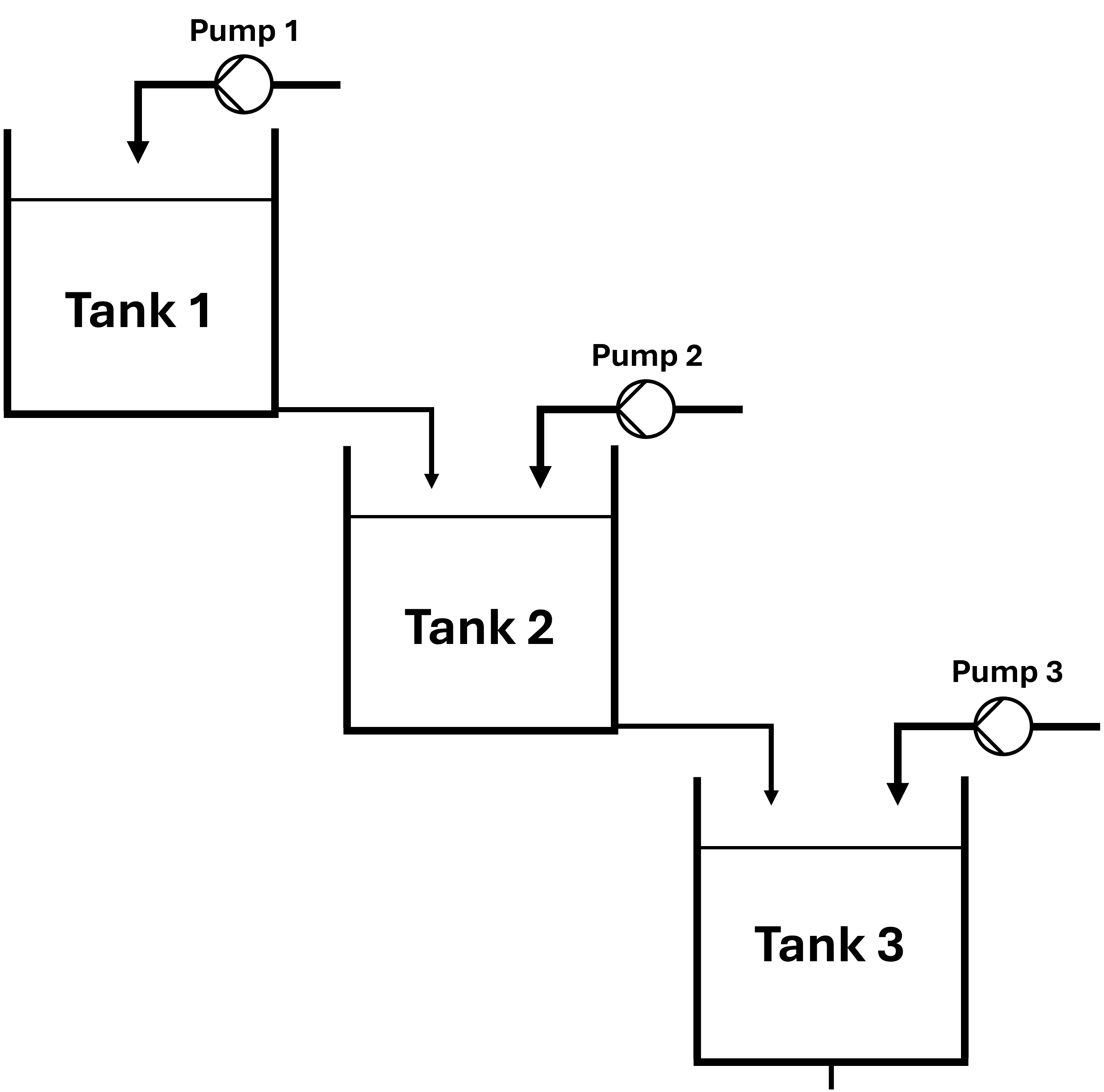
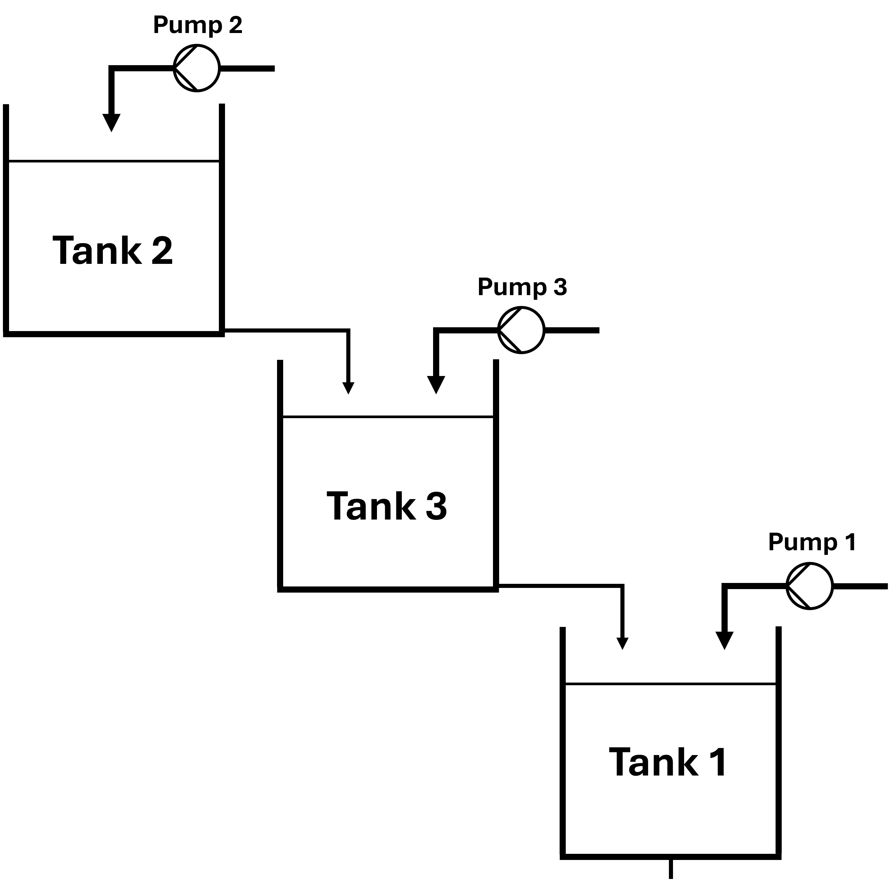
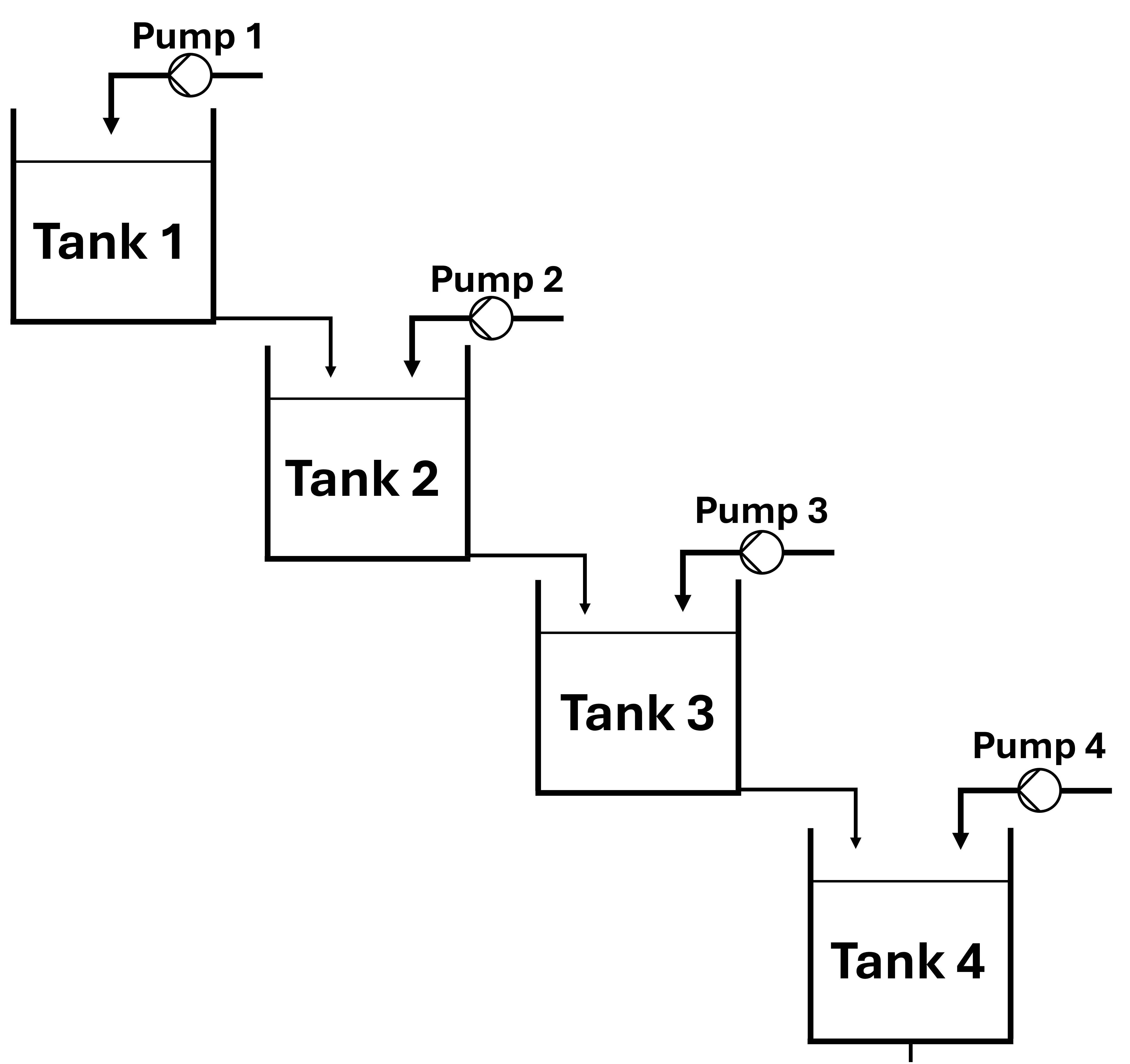
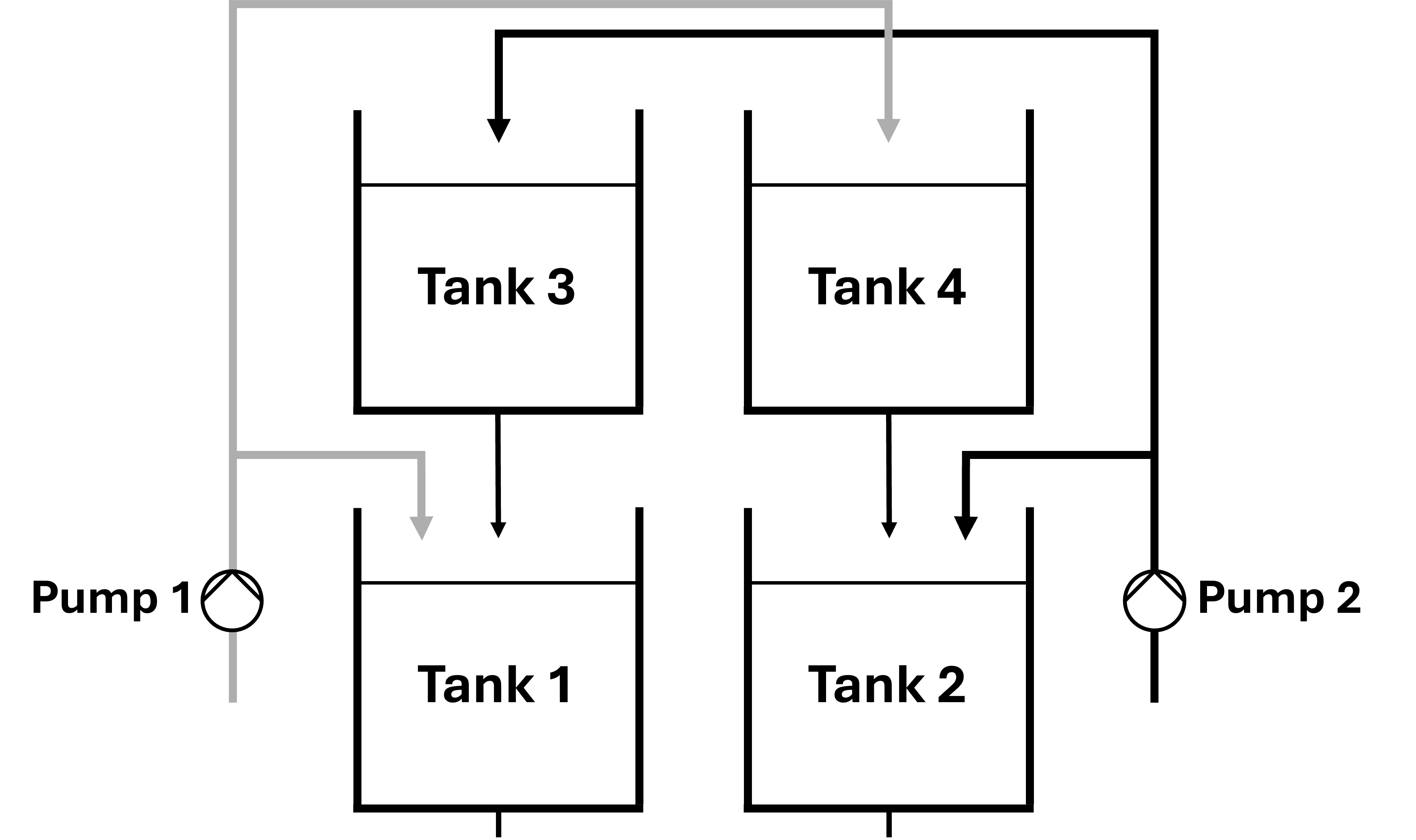
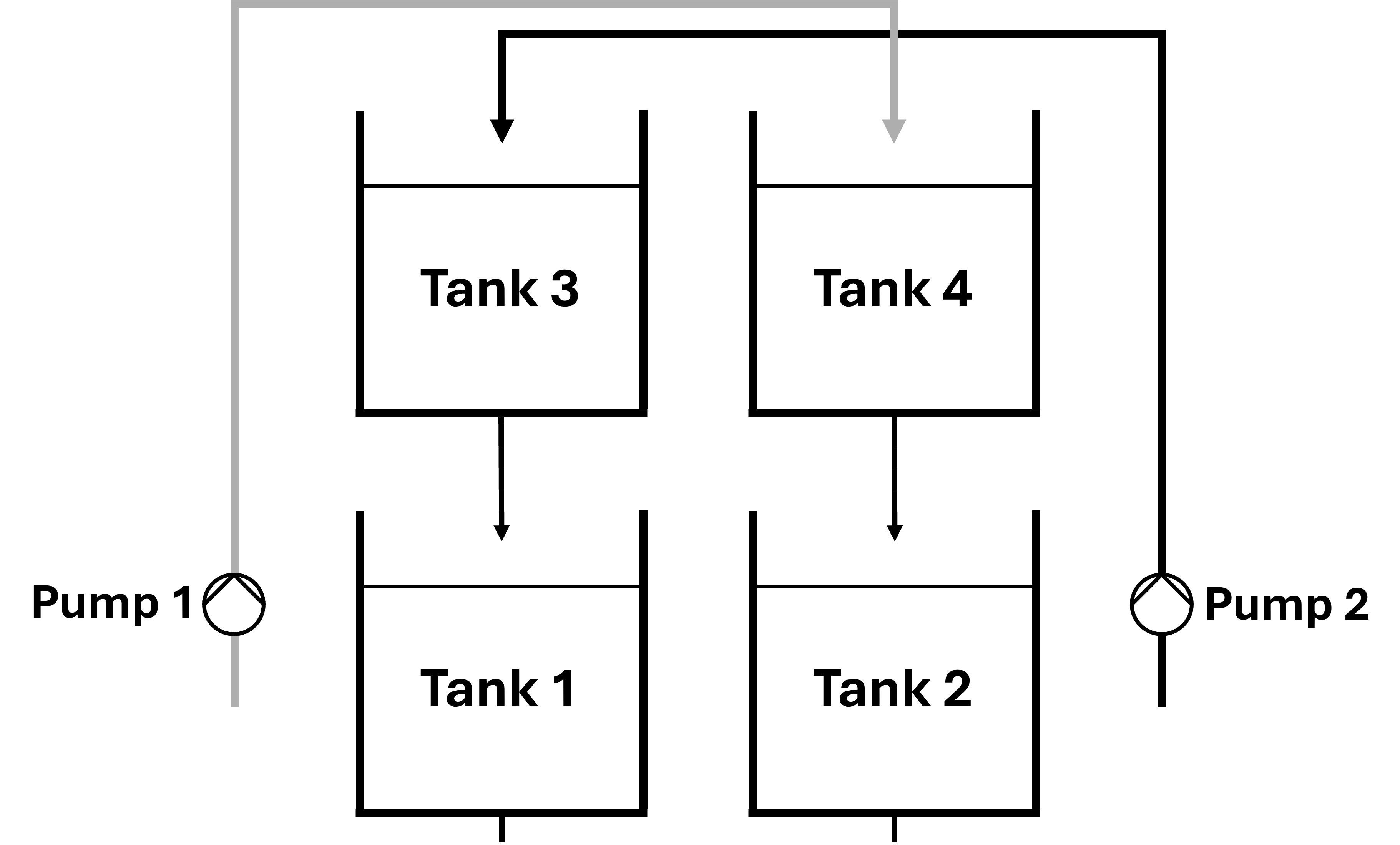

Finally, we evaluate the performance of tuned controllers following different stage definitions. We evaluate the performance for three benchmarks: (1) two cascaded tanks, (2) three cascaded tanks, (3) four cascaded tanks. Tank labeling is not relevant in the case of control performance evaluation.
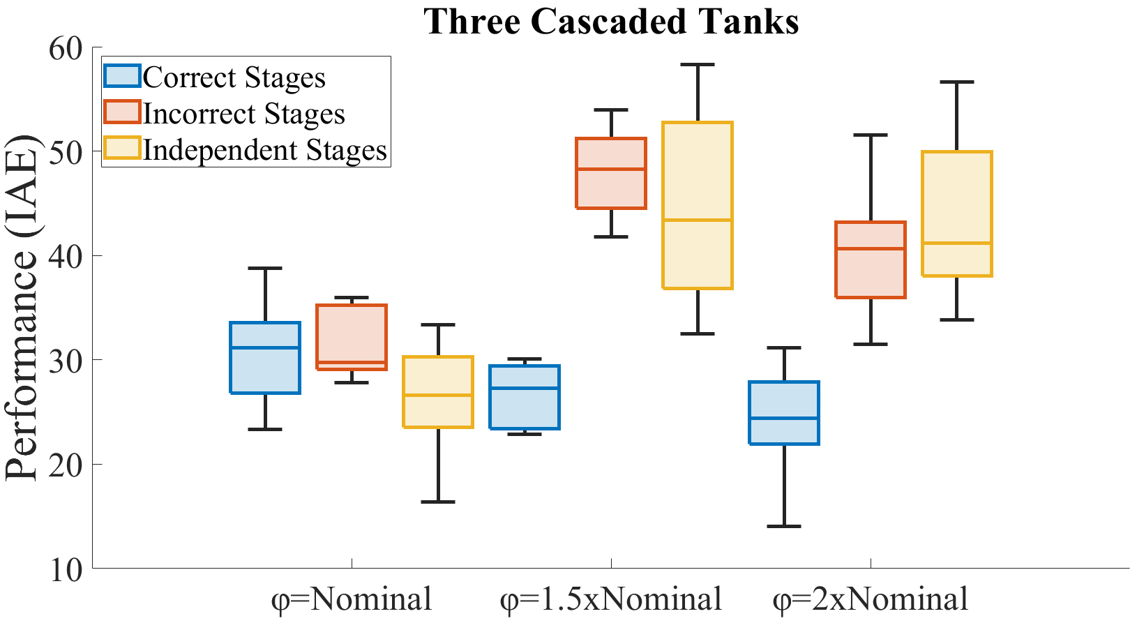
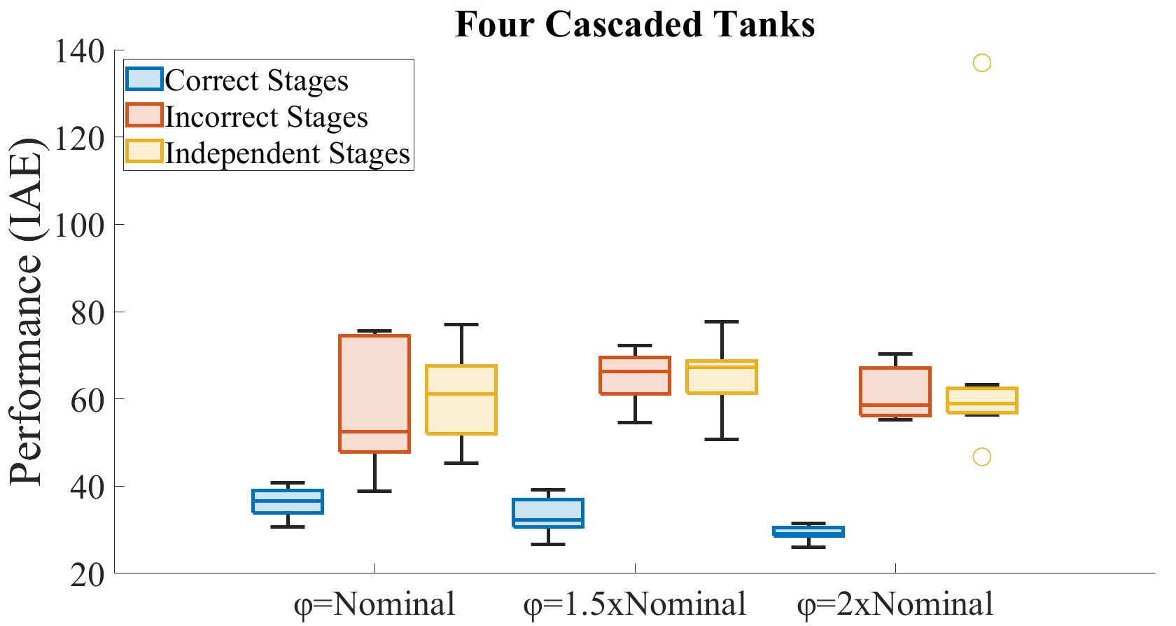
Controller performance is evaluated for different levels of coupling. For this purpose, we define a coupling parameter that represents how coupled the control loops in the system are. For the case of the cascaded configurations used, we model the coupling parameter as a factor that linearly maps the diameters of the drain in the tanks. A high value of results in a larger drain diameter, which results in higher drain flows for each tank, which in turn results in higher input flows into the respective tanks below, translating into higher coupling between tanks. Conversely, a small drain diameter might result in practically non-existent coupling between the tanks, which would result in a set of isolated control loops, rendering the motivation for proper stage definition null. We evaluate the controller performance for three coupling levels: nominal coupling and 1.5 and 2 times nominal coupling.
Three stage definitions are evaluated, labeled: correct stage definition, incorrect stage definition, and independent stage definition. Correct stage definition for the three cascaded configurations refers to a solution that tunes the control loops following the hierarchy; i.e.: the control loop for the tank on top is tuned first, then the tank below, and so on until the bottom tank is reached, while at each stage, control loops tuned in previous stages are closed and controllers are fixed to their tuned parameters. Incorrect stage definition refers to a solution that tunes control loops in the opposite order to the correct stage definition while maintaining control loops from previous stages closed. Independent stage definition refers to the process of tuning a control loop independently at each stage, ie.: control tunings from previous stages do not carry over to the current stage and every loop, except the loop being tuned, is open at each stage. The tuning order in this case is not important. This is technically also an incorrect stage definition for the cascaded configurations, however, we include it as a separate case because it is a common approach to controller tuning in the related literature [2][12]. Fig. 10 shows example stage definitions for the two cascaded tanks system.
6 Results and Discussion
In this section we empirically validate the proposed methodology and evaluate the I/O pairing and stage definition tasks for multiple configurations of the multi-tanks system, using performance metrics discussed in the previous section. All LLM experimental results were produced using the Claude-Sonnet-3.7 and Claude-Sonnet-4 LLMs, accessed via Anthropic API [1]. The temperature parameter for the API calls was set to 1.0, which promotes stochasticity and variety in the LLM outputs. The associated codebase and results can be found at https://github.com/mjares/DX2025_LLMs_ExpertKnowledge.git.
6.1 Input-Output Pairing
To evaluate the performance of the LLM-based methodology when proposing I/O pairings in a given system, we consider the benchmarks described in Section 5.2. Every input-system prompt pair was evaluated times and percentage values were reported. Overall, we can see in Table 1 that the performance was high across all metrics, with 100% consistency in terms of formatting, which is a challenging task. Accuracy was also high at over 98% for all cases. This empirically shows that an LLM-based solution can yield expert knowledge recommendations regarding I/O pairing for benchmarks within the family of multi-tank systems. Furthermore, for the case of the benchmarks taken from [12], the I/O pairing matches the one achieved by the optimization approach with over 98% accuracy, while requiring less resources in terms of optimization problem formulation, expert interactions, and, potentially, computational cost (assuming inference cost from an LLM interaction is lower than the cost from solving the optimization problem).
| Benchmark | Correct Format (%) | Accuracy (%) | Accuracy/Format (%) | |||
|---|---|---|---|---|---|---|
| Sonnet3.7 | Sonnet4 | Sonnet3.7 | Sonnet4 | Sonnet3.7 | Sonnet4 | |
| (1): (3T, 1a2, 2a3) | 100 | 100 | 100 | 100 | 100 | 100 |
| (2): (4T, 1a2, 2a3, 3a4) | 100 | 100 | 100 | 100 | 100 | 100 |
| (3): (4T, 1b3, 2b4)[12] | 100 | 100 | 100 | 98 | 100 | 98 |
| (4): (4T, 1b3, 2b4)* | 100 | 100 | 99 | 100 | 99 | 100 |
| (5): 1T Temperature [12] | 100 | 100 | 98 | 100 | 98 | 100 |
6.2 Stage Definition
In order to evaluate the performance of the LLM-based methodology to define stages for a multistage control tuning framework, we consider the system configurations described in Section 5.2. Each input-system prompt pair was evaluated times and percentage values were reported. Table 2 shows a summary of the performance. While formatting was not as consistent as the I/O pairing case, we can see a very high accuracy/formatting metric with 100% accuracy in most benchmarks. As discussed in Section 5.1.1, accuracy/formatting should be the priority metric, since incorrect formatting can be automatically detected, repeating the interaction with the LLM until a correctly formatted output is produced.
| Benchmark | Correct Format (%) | Accuracy (%) | Accuracy/Format (%) | |||
|---|---|---|---|---|---|---|
| Sonnet3.7 | Sonnet4 | Sonnet3.7 | Sonnet4 | Sonnet3.7 | Sonnet4 | |
| (1): (2T, 1a2) | 98 | 100 | 98 | 99 | 100 | 99 |
| (2): (2T, 1b2) | 97 | 100 | 97 | 100 | 100 | 100 |
| (3): (2T, 1-2ic) | 100 | 100 | 100 | 100 | 100 | 100 |
| (4): (3T, 1a2, 2a3) | 93 | 100 | 93 | 100 | 100 | 100 |
| (5): (3T, 1b3, 2a3) | 96 | 100 | 96 | 100 | 100 | 100 |
| (6): (3T, 1a3, 2-3ic) | 96 | 100 | 94 | 98 | 97.9 | 98 |
| (7): (4T, 1a2, 2a3, 3a4) | 94 | 100 | 94 | 100 | 100 | 100 |
6.2.1 Comparing performance of tuned controllers for different stage definitions
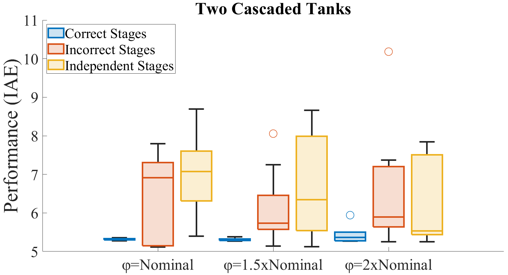
In this section, we empirically compare the performance of tuned controllers described in Section 5.2. Controllers are tuned times for every combination of system configuration, coupling level, and stage definition, and box-plot results over the 10 runs are reported in Fig. 11. Performance is measured in integral absolute error (IAE), and lower error values are desired. Overall, we can see that, as the complexity of the system increases, i.e.: input-output space dimensions, number of components (tanks), etc., the impact of the stage definition on performance increases. In Fig. 11(c), which is the most complex system evaluated (four cascaded tanks), there is a distinct difference between the performance achieved when following the correct stage definition and the incorrect stage definitions; however, for the lower complexity benchmarks (Figures 11(a) and 11(b)) the difference is not obvious, with the two cascaded tank system showing the largest overlap between stage definitions. Similarly, for every benchmark, an increase in coupling (represented by the parameter) is also associated with higher differences between the performances achieved under the correct and incorrect stage definitions; this is an expected result, as stated in Section 5.2. When we compare performance improvement for the three tank benchmark, we can see there is a significant performance improvement when the coupling in the system is high, but there is barely any difference between stage definitions when the coupling is lower. In general, the greatest improvement can be seen for the four cascaded tank benchmark at 2 times nominal coupling (Figure 11(c)) where a correct stage definition can reduce the error of the tuned controllers by 52% with respect to the incorrect stage definitions.
6.3 Discussion, Limitations, and Future Works
We have evaluated the proposed methodology for a variety of multi-tank benchmarks (Figures 7, 8, and 9), including a benchmark where temperature and level in a tank are controlled simultaneously (Fig. 9(c)), and a set of cascading tank benchmarks with different levels of coupling (Fig. 11). We have empirically shown that, for these benchmarks, stage definition can have significant impact on the performance of the tuned controllers. Furthermore, we have shown that the proposed methodology for stage definition using LLMs can propose the correct stage definition and I/O pairing with a high degree of consistency and accuracy.
We acknowledge that, even though the actuator label space () can integrate notions of temperature control, as well as other potential extensions (e.g.: liquid composition/concentration), the proposed methodology is mostly centered around the problem of level control in a family of systems consisting of reservoirs, pumps, and connections. In spite of this limitation, this is a first step towards a system-informed general methodology for prompt engineering with the purpose of expert knowledge automation. An extension of these results to a wider variety of benchmarks would require a redefinition of the mathematical language and the prompt engineering algorithm; however, the core elements of the methodology would persist: a graph representation of the system components and interactions, and a prompt engineering algorithm that binds this graph language to the input prompt space of an LLM. Future works should focus on proposing a generalized mathematical language and prompt engineering algorithm, or, if this is not possible, a set of general guidelines for developing these graph representations and prompt engineering algorithms for different families of benchmarks.
We have proposed a simple topology-based graph representation of the system since we are aiming for a solution that requires minimal expert interaction and knowledge of the system, which would be a limitation for more complex system representations such as bond graphs, process graphs, or structural analysis. However, a generalization of this methodology for systems other than the multi-tank benchmarks will most likely require more complex representations of the system, such as the ones mentioned above.
We have focused on systems with centralized control since I/O pairing and stage definition for sequential controller tuning would rarely be relevant in a centralized control approach. Furthermore, decentralized parametric controllers, or a hybrid between decentralized and supervisory control are industry standard solutions. However, future works should focus on extending the methodology to consider systems with centralized/supervisory control, as well as systems with integrated decoupling strategies.
This work is also limited by the lack of formal definition of what is a correct I/O pairing or stage definition apart from what is referenced as expert knowledge in the associated literature. Therefore, future works will provide a formal framework to measure validity of expert knowledge in terms of I/O pairing and stage definition.
7 Conclusions
This paper addresses controller-tuning aspects of automated engineering system design. We proposed a mathematical language to describe a family of multi-tank benchmarks based on system topology. We implemented an algorithm to bind this mathematical language to the input prompt space of a Large Language Model as a form of prompt engineering. Following this methodology, we automated expert knowledge requirements in decentralized controller auto-tuning related to I/O pairing and stage definition for a multistage tuning framework. Our proposed methodology showed an accuracy of over 97% for both I/O pairing and stage definition, with consistent output formatting. Furthermore, we empirically evaluated the performance of tuned controllers for different stage definitions in a family of multi-tank benchmarks and showed that, depending on the complexity of the system, and degree of coupling between control loops, a correct stage definition can improve performance over the incorrect stage definitions by up to 52%. Future works will extend the mathematical language and the prompt engineering algorithm to a wider variety of benchmarks.
References
- [1] Anthropic api. URL: https://console.anthropic.com.
- [2] Marlon J. Ares-Milian, Gregory Provan, and Marcos Quinones-Grueiro. Towards automated controller parameter design in cyber-physical systems: Improving computational cost. In 2025 IEEE International Conference on Smart Computing, SMARTCOMP 2025, 2025.
- [3] Aman Bhargava, Cameron Witkowski, Shi-Zhuo Looi, and Matt Thomson. What’s the magic word? a control theory of llm prompting, October 2023. doi:10.48550/arXiv.2310.04444.
- [4] B. Ould Bouamama, G. Biswas, R. Loureiro, and R. Merzouki. Graphical methods for diagnosis of dynamic systems: Review, 2014. doi:10.1016/j.arcontrol.2014.09.004.
- [5] Tom B Brown, Benjamin Mann, Nick Ryder, and Melanie Subbiah et. al. Language models are few-shot learners. In NeurIPS 2020, 2020.
- [6] Y. Chen, R. Goebel, G. Lin, B. Su, Y. Xu, and A. Zhang. An improved approximation algorithm for the minimum 3-path partition problem. Journal of Combinatorial Optimization, 38:150–164, 2019. doi:10.1007/s10878-018-00372-z.
- [7] Xingang Guo, Darioush Keivan, Usman Syed, Lianhui Qin, Huan Zhang, Geir Dullerud, Peter Seiler, and Bin Hu. Controlagent: Automating control system design via novel integration of llm agents and domain expertise. arXiv preprint arXiv:2410.19811, 2024. doi:10.48550/arXiv.2410.19811.
- [8] P. Hehenberger, B. Vogel-Heuser, D. Bradley, B. Eynard, T. Tomiyama, and S. Achiche. Design, modelling, simulation and integration of cyber physical systems: Methods and applications. Computers in Industry, 82:273–289, October 2016. doi:10.1016/j.compind.2016.05.006.
- [9] H J Kushner. A new method of locating the maximum point of an arbitrary multipeak curve in the presence of noise. Journal of Basic Engineering, 1964.
- [10] Jiang Lu, Pinghua Gong, Jieping Ye, Jianwei Zhang, and Changshui Zhang. A survey on machine learning from few samples, September 2020. arXiv:2009.02653.
- [11] Yifan Luo, Yiming Tang, Chengfeng Shen, Zhenan Zhou null, and Bin Dong. Prompt engineering through the lens of optimal control. Journal of Machine Learning, 2:241–258, January 2023. doi:10.4208/jml.231023.
- [12] Vasileios K. Mappas, Vassilios S. Vassiliadis, Bogdan Dorneanu, Alexander F. Routh, and Harvey Arellano-Garcia. Automated control loop selection via multistage optimal control formulation and nonlinear programming. Chemical Engineering Research and Design, 195:76–95, July 2023. doi:10.1016/j.cherd.2023.05.041.
- [13] Sammyak Mate, Pawankumar Pal, Anshumali Jaiswal, and Sharad Bhartiya. Simultaneous tuning of multiple pid controllers for multivariable systems using deep reinforcement learning. Digital Chemical Engineering, 9, December 2023. doi:10.1016/j.dche.2023.100131.
- [14] Silke Merkelbach, Alexander Diedrich, Anna Sztyber-Betley, Louise Travé-Massuyès, Elodie Chanthery, Oliver Niggemann, and Roman Dumitrescu. Using multi-modal llms to create models for fault diagnosis. In The 35th International Conference on Principles of Diagnosis and Resilient Systems (DX’24), volume 125, November 2024. doi:10.4230/OASIcs.DX.2024.6.
- [15] C. E. Rasmussen and C. K. I. Williams. Gaussian Processes for Machine Learning. USA:MIT Press, January 2006.
- [16] Alejandro Rodríguez-Molina, Efrén Mezura-Montes, Miguel G. Villarreal-Cervantes, and Mario Aldape-Pérez. Multi-objective meta-heuristic optimization in intelligent control: A survey on the controller tuning problem. Applied Soft Computing Journal, 93, August 2020.
- [17] D. Stenger, M. Nitsch, and D. Abel. Joint constrained bayesian optimization of planning, guidance, control, and state estimation of an autonomous underwater vehicle. In ECC 2022, 2022.
- [18] Prerit Terway, Kenza Hamidouche, and Niraj K. Jha. Dispatch: Design space exploration of cyber-physical systems, September 2020. arXiv:2009.10214.
- [19] K. Tohma, H. İ. Okur, H. Gürsoy-Demir, M. N. Aydn, and C. Yeroğlu. Smartcontrol: Interactive pid controller design powered by llm agents and control system expertise. SoftwareX, 31:102194, 2025. doi:10.1016/J.SOFTX.2025.102194.
- [20] Collin Zhang, John X. Morris, and Vitaly Shmatikov. Extracting prompts by inverting llm outputs, May 2024. doi:10.48550/arXiv.2405.15012.