Beyond Dynamic Bayesian Networks: Fusing Temporal Logic Monitors with Probabilistic Diagnosis
Abstract
Conventional diagnostic systems often fail to account for temporal dynamics – such as duration, frequency, or sequence of events – which are critical for accurate fault assessment. Existing solutions that model time, like Dynamic Bayesian Networks (DBNs), typically suffer from computational complexity and scalability issues.
This paper introduces a hybrid diagnostic architecture that integrates a standard Bayesian Networks (BNs) with a powerful temporal reasoner R2U2 (Realizable Responsive Unobtrusive Unit). By decoupling temporal logic from probabilistic inference, our approach allows the specialized R2U2 engine to efficiently process complex time-dependent conditions and provide nuanced inputs to the BNs. The result is a more scalable, flexible, and robust framework for diagnosing failures in systems where temporal behavior is a key factor. The paper will detail this architecture, its generation from system models, and demonstrate its capabilities using a UAV electric powertrain example.
Keywords and phrases:
Bayesian diagnostic network, temporal logic, fault diagnosis, temporal reasoning, probabilistic inference, scalabilityCategory:
Short PaperCopyright and License:
2012 ACM Subject Classification:
Computing methodologies Causal reasoning and diagnostics ; Computing methodologies Temporal reasoning ; Mathematics of computing Probabilistic inference problems ; Computing methodologies Multiscale systems ; Mathematics of computing Bayesian networksAcknowledgements:
This work was authored by employees of KBR Wyle Services, LLC under Contract No. 80ARC020D0010 with the National Aeronautics and Space Administration. The United States Government retains and the publisher, by accepting the article for publication, acknowledges that the United States Government retains a non-exclusive, paid-up, irrevocable, worldwide license to reproduce, prepare derivative works, distribute copies to the public, and perform publicly and display publicly, or allow others to do so, for United States Government purposes. All other rights are reserved by the copyright owner.Editors:
Marcos Quinones-Grueiro, Gautam Biswas, and Ingo PillSeries and Publisher:
1 Introduction
The ability to diagnose and resolve system malfunctions at their source is fundamental to the reliability of any complex domain, a critical capability delivered by a robust diagnostics framework. Although the term is frequently used interchangeably with Fault Detection and Isolation (FDI), diagnostics is a distinct discipline; whereas FDI is concerned with the identification and localization of a fault, diagnostics endeavors to determine the precise nature and underlying cause of said failure. A comprehensive array of methodologies has been developed to this end, spanning from elementary D-matrices that map test outcomes to failure modes, to more sophisticated probabilistic models like Bayesian Networks (BNs) and data-driven techniques such as Deep Neural Networks (DNNs). These approaches are broadly classifiable as either model-based, which depend on an explicit representation of the system, or model-free, which derive their logic from empirical data. Moreover, the field of diagnostics is intrinsically linked with system safety and reliability disciplines, such as Fault Tree Analysis (FTA) and Failure Mode and Effects Analysis (FMEA), frequently serving as the mechanism for the practical detection of failure modes identified therein.
A considerable limitation inherent in many conventional diagnostic methodologies is their static character; while effective in representing the direct causal relationships between signals and failure modes, they inadequately incorporate temporal dynamics. These temporal considerations are, however, often indispensable for an accurate diagnosis. For example, a transient voltage fluctuation may be considered insignificant, yet the same condition constitutes a valid fault if it persists for a specified minimum duration. Likewise, subsequent to a change in a system’s operational mode, certain error conditions may be anticipated and must be disregarded for a defined interval to preclude erroneous fault indications. Other temporal patterns, such as the occurrence frequency of anomalous data packets or the specific sequence of events, can alter the diagnostic output. Although solutions like Dynamic Bayesian Networks (DBNs) attempt to model these time-dependent relationships, their application is often hindered by computational complexity and model size, which increases as the network is unrolled over time, and they exhibit limitations in efficiently managing disparate temporal intervals.
To surmount these challenges, a hybrid R2U2/BN diagnosis system is proposed for advanced model-based temporal diagnosis. This framework integrates three principal components: a standard diagnostic Bayesian Network, a high-capability temporal reasoner (R2U2), and the potential for incorporating requirements specified in natural language. The novelty of this approach resides in the symbiotic integration wherein the BN’s inputs (test signals) and its outputs (health-state nodes) serve as inputs for the R2U2 reasoner. This reasoner, in turn, supplies temporally processed information to the BN. This architecture facilitates robust temporal pre-processing, enabling the formulation of complex logical conditions, or “temporal tests,” such as “the voltage remained below a threshold for at least 10 seconds” or “the lidar system’s health metric was below 0.7 for a minimum of 2 seconds.” The R2U2 component employs synchronous observers for Future Time Logic (FTL) that utilize a three-valued logic (true, false, maybe). When propagated to the BN, this three-valued input provides more nuanced insights for diagnostic reasoning, thereby overcoming the scalability and interval-management deficiencies characteristic of DBNs.
The motivation for this hybrid architecture arises from the inherent limitations of DBNs. By embedding temporal relationships directly into the probabilistic graph, DBNs suffer from state-space explosion and computational intractability, which complicates modeling sophisticated temporal patterns. The proposed R2U2/BN system provides a more scalable solution by decoupling temporal reasoning from probabilistic inference. This separation of concerns allows the Bayesian Network to remain a compact model of causal failures, while the specialized R2U2 reasoner efficiently handles the full expressive power of temporal logic. The resulting framework is therefore more flexible and robust for diagnosing systems where complex temporal dynamics are a critical component of the process.
The rest of this paper systematically develops our proposed diagnostic architecture. Section 2 provides the necessary background on diagnostic Bayesian networks and the R2U2 monitoring engine. With this foundation, Section 3 introduces our novel methodology, explaining how we combine temporal monitors with Bayesian networks and how these models are generated from FMEA. We then provide context by comparing our work to existing research in Section 4, before offering a final summary and outlining future research avenues in Section 5.
2 Background
2.1 Diagnostic Bayesian Networks
As defined by Pearl [22], Bayesian Networks (BNs) are directed acyclic graphs that model causal relationships between variables. In this framework, the nodes represent the variables themselves, while the connecting arcs point from a cause to its direct effect. The probabilistic strength of these causal links is captured by conditional probabilities. The example below, also from [22], serves as a practical illustration of a BN in action.
Figure 1 shows a representative BN, where the complete joint probability distribution is the product of the conditional probabilities of each proposition given its ancestors, Eq. (1).
| (1) |
The joint probability distribution could also be expressed with the following notation:
| (2) |
where represents the set of ancestors of variable , and is the random vector containing all variables [23, 2]. For example, the term becomes .
Dependencies among propositions are described through the definition of sets of ancestors (or parents) and descendants (or children). For example, the set contains the ancestors of , while contains the children of . This structural model allows analysis over interventions, i.e., enable the computation of the joint probability density function (pdf) conditioned on some specific assumptions over a specific variable in the network [23]. Starting from the example in Figure 1, it is possible to evaluate the joint pdf given, e.g., has been defined True:
| (3) |
A key challenge in applying Bayesian Networks is the effort required to assess all conditional probabilities. Each node in the network needs a Conditional Probability Table (CPT) that defines its state based on every possible combination of its parents’ values, meaning the table’s size grows combinatorially with the number of parents. For instance, while we can represent an intervention like forcing by simply removing the edge from its parent (as its state no longer depends on , see Eq. (3)), the initial construction of such dependency tables for networks with many interconnected nodes remains a significant practical obstacle.
2.2 The R2U2 Monitoring Engine
The real-time R2U2 (Realizable, Responsive, and Unobtrusive Unit) has been developed to continuously monitor system and safety properties of an aerospace system. R2U2 has been implemented as an FPGA configuration [10]. and a software component. Hierarchical and modular models within this framework [27, 28] are defined using Metric Temporal Logic (MTL) [13] and mission-time Linear Temporal Logic (LTL) [25] for expressing Boolean formulas and temporal properties. In the following, we give a high-level overview over the R2U2 framework and its implementation. For details on temporal reasoning, its implementation, and semantics the reader is referred to [25, 10, 28].
2.2.1 Temporal Logic Observers
LTL and MTL formulas consist of propositional variables, the logic operators , , , or , and temporal operators to express temporal relationships between events.
R2U2 is capable of handling formulas for the past-time fragment of temporal logic as well as future time. Below, we briefly describe future-time operators and their informal semantics. For LTL formulas , we have (), (), (), (), and (). Their formal definition and concise semantics is given in [25]. On an informal level, given Boolean variables , , the temporal operators have the following meaning (see also Figure 2):
-
() means that must be true at all times along the timeline.
-
() means that must be true at some time, either now or in the future.
-
() means that must be true in the next time step; in this paper a time step is a tick of the system clock aboard the UAV.
-
() signifies that either is true now, at the current time, or else is true now and will remain true consistently until a future time when must be true. Note that must be true sometime; cannot simply be true forever.
-
() signifies that either both and are true now or is true now and remains true unless there comes a time in the future when is also true, i.e., is true. Note that in this case there is no requirement that will ever become true; could simply be true forever. The Release operator is often thought of as a “button push” operator: pushing button triggers event .
| LTL Op | Timeline |
| MTL Op | Timeline |
|---|---|
For MTL, each of the temporal operators are accompanied by upper and lower time bounds that express the time period during which the operator must hold. Specifically, MTL includes the operators , , , and , where the temporal operator applies over the interval between time and time , inclusive (Figure 2).
Additionally, we use a mission bounded variant of LTL [25] where these time bounds are implied to be the start and end of the mission of a UAV. Throughout this paper, time steps corresponds to ticks of the system clock. So, a time bound of would designate the time bound between 0 and 7 ticks of the system clock from now. Note that this bound is relative to “now” so that continuously monitoring a formula would produce true at every time step for which holds anytime between and time steps after , and false otherwise.
3 Temporal Bayesian Diagnosis with Temporal Logic Monitors
Our approach for diagnostic reasoning with temporal elements is based upon the synergistic combination of an efficient reasoning algorithm for Bayesian networks and the R2U2 temporal engine.
3.1 Tool Architecture and Modeling Process
Figure 3 gives a high-level overview of the architecture for our approach. Input signals , which are obtained at time point from sensors, software sensors, the system status, and outputs of our diagnostic BN are first going through a signal processing stage, where the values, usually floating point numbers, are scaled and subjected to thresholding to obtain Boolean values. In our architecture, the thresholds and range limits are model-based and assumed to be fixed. For example, a floating point signal might be thresholded using to obtain the Boolean value Ubatt_low. Signal processing is carried out with a fixed basic rate, e.g., 10Hz.
The vector of Boolean values for time are now input to the R2U2 monitoring engine. Here, formulas in past-time and future-time logic are evaluated to yield Boolean or 3-valued (see Section 3.5.1) valuations of each of the formulas at . These outputs comprise the output of our diagnostic system and are also fed into the diagnostic BN.
For example, the formula could correspond to a failure-mode “battery-too-weak-unusable”. On the other hand, a formula would filter out short drops or glitches of the battery voltage, and the result would be used as a value for an observable sensor node in the BN.
At each point in time , the BN is evaluated and posterior probabilities are calculated. These probabilities for selected nodes correspond to the presence of failure modes or can correspond to component health; these values are direct outputs for our diagnosis system.
These posterior probabilities can also provide valuable information, when considered over time: for example, knowing if subsystem has a poor health for an extended period of time. Therefore, selected values are fed back into the signal processing to be able to formalize such temporal properties.
| Model | Context | Description |
|---|---|---|
| Effect | Fault Propagation Model | Functions cross referenced in fault propagation model. This is used to capture the functional degradation due to the presence of one or more fault(s). |
| Implementation | Functional Decomposition Model | Reference to blocks in the system model that implement one or more function(s) in the functional decomposition model. |
| Ambiguity Set | Fault Impact, Refinement Model | Represents a set of faults which cannot be distinguished based on the triggering Tests. |
| Operational Impact | Fault Impact, Recovery Plan | Reference to system variables and changes in their operating range. |
| Requirement | Active Diagnosis Procedures, Recovery Plan | Conditions on system variables in order to execute active diagnosis procedures or recovery plans. |
| Mode Requirement | Active Diagnosis Procedures, Recovery plan | Conditions on system modes in order to execute active diagnosis procedures or recovery plans. |
| TestRefs | Active Diagnosis Procedures | Additional tests that can be evaluated when an active diagnosis procedure is executed. |
| Trigger Condition | Recovery Plan | A set of faults related to triggering a recovery plan. Any of the faults in the triggering condition may be handled using the recovery plan. |
| Mode Change | Recovery Plan | Mode change introduced by executing a recovery plan. |
Our proposed diagnostic architecture is purely model-driven and contains no machine-learning elements. The process steps for configuring and tailoring our tool is outlined in Figure 4. We derive diagnostic information from a comprehensive suite of models that are developed during the design phase of a complex and potentially autonomous system (see Table 1 for an overview). Most notably, functional decomposition models, fault trees, and the outputs of a Failure Mode and Effects Analysis (FMEA) are used to automatically construct the diagnostic Bayesian Network. The probabilities for the Bayesian transitions are informed by a combination of metrics, including Mean Time To Failure (MTTF) and Mean Time Between Failures (MTBF), as well as operational conditions, system health, and subject matter expert (SME) expertise.
These models, together with system and component requirements, Concept of Operations (ConOPS), and safety/performance requirements are used to define the logic and temporal monitors for R2U2. In the following sections, we describe in detail how the BN and temporal monitors are constructed, before we discuss a realistic example.
3.2 BN Construction from Failure Mode and Effects Analysis (FMEA)
To develop an effective system-level diagnosis framework under uncertain conditions, we integrate information from a Failure Mode and Effects Analysis (FMEA) with a Bayesian Network (BN). This process unfolds in two main stages: first, we construct the graphical structure of the BN, and second, we define its conditional probability tables (CPTs) which quantify the relationships between different failure events.
The initial stage involves building the network’s structure by translating the qualitative FMEA data into the BN’s components. Then systematically convert the identified causes, failure modes, and effects from the FMEA into nodes within the network. This includes creating “observable” nodes that represent real-world sensor data – such as a high-temperature reading – which are critical for identifying and isolating the root cause of a failure. The network is then assembled by drawing directed arcs that reflect the causal logic from the FMEA, pointing from causes to their resulting failure modes and from failure modes to their ultimate effects. A simple example of a BN structure build from FMEA of an UAV electric powertrain is shown in Fig.5 for illustration.
With the Bayesian Network (BN) structure in place, we then assign probabilities to each node. First, root nodes (those with no parent nodes) are given prior marginal probabilities. Next, every other node is assigned a conditional probability based on its parent nodes, using information derived from the FMEA. To determine these values, we can draw from several sources, including historical failure data, the expertise of engineers, or established techniques such as maximum entropy theory [11].
Once the BN is fully defined, it can be used to detect and localize a fault within a complex system by turning observable nodes to True or False. The process starts when an observable evidence node, or “symptom,” is triggered – for example, when a sensor value exceeds a set threshold. This new evidence is fed into the network, which then uses Bayesian inference to update the probability of every potential root cause. The cause that emerges with the highest failure probability is identified as the source of the fault. We will address potential complicating factors, such as environmental conditions and false alarms, in the next section.
3.3 Detailed Modeling Approach and Issues
The dependency among elements in FMEAs do not have to be restricted to deterministic relationships in BNs [2], and this property intrinsically enhances the modeling of the diagnostic system. Let us consider, for simplicity, a fault event with two root causes, its ancestors, and . Table 2 is the conditional probability table of the model, where probabilities are defined through three binary subscripts . The term defines the probability of the outcome given values , with referring to the fault event and referring to its ancestors and . For example, is the probability that given both ancestors are 0 (or False).
| 0 | 0 | ||
|---|---|---|---|
| 0 | 1 | ||
| 1 | 0 | ||
| 1 | 1 | ||
The fault event may happen, with low probability, because of external causes or unknown events not described by its ancestors. Such external forcing was called Common Cause Failures in [2], and following that idea, , and so . On the opposite side of the spectrum, the fault event may not happen even if both ancestors are activated (true). This option describes the ability of a system to work partially or reconfigure, [2], or describes a statistical relationship between the three elements, suggesting that root causes do not deterministically trigger the failure, so . As a result, the two ancestors may occur without triggering the fault event, so and . Different ancestors may influence the fault event in different ways, e.g. according to the severity of the root cause. This properties can be easily embedded in the network by assigning different values to the probabilities conditioned over and .
In addition to the cases of failures induced by external variables or prevented system reconfiguration, the BN should also account for the performance of the measuring and/or detection system. In the proposed architecture, the evidence used to perform inference over the network is collected through sensors that measure variables connected (directly or indirectly) to the fault event we aim to detect. The sensor performance or, similarly, the ability of the detection system to identify anomalous sensor data, should be embedded in the estimation of the CPT values. Reconnecting to the previous example, therefore, the element in Table 2 should account for false alarm rates, and should include, on top of any statistical relationship between the elements, the probability of mis-detection.
3.4 Efficient Evaluation of BN
Different BN inference algorithms can be used to compute a posterior probabilities. These algorithms include junction tree propagation [14, 12, 29] conditioning [8], variable elimination [17, 30], stochastic local search [21, 19], and arithmetic circuit evaluation [9, 5].
We select arithmetic circuit (AC) evaluation as our inference algorithm, which compiles our diagnostic BN into an arithmetic circuit. Especially for real-time aerospace systems, where there is a strong need to align the resource consumption of diagnostic computation to resource bounds [20, 18] algorithms based upon arithmetic circuit evaluation are powerful, as they provide predictable real-time performance [5]. An arithmetic circuit is a directed acyclic graph (DAG) in which the leaf nodes represent parameters and indicators while other nodes represent addition and multiplication operators. Figure 6 shows a small BN and its corresponding AC.
A B
Posterior marginals in a Bayesian Network can be computed from the joint distribution over all variables :
where are the parameters of the Bayesian network, i.e., the conditional probabilities that a variable is in state given that its parents are in the joint state , i.e., . Further, indicates whether or not state is consistent with BN inputs or evidence. For efficient calculation, we rewrite the joint distribution into the corresponding network polynomial [9]:
An arithmetic circuit is a compact representation of a network polynomial [7] which, in its in-compact form, is exponential in size and thus unrealistic in the general case. Hence, answers to probabilistic queries, including marginals and most probable explanations (MPEs), are computed using algorithms that operate directly on the arithmetic circuit. The marginal probability (see Corollary 1 in [9]) for given evidence is calculated as
where is the probability of the evidence . In a bottom-up pass over the circuit, the probability of a particular evidence setting (or clamping of parameters) is evaluated. A subsequent top-down pass over the circuit computes the partial derivatives .
To evaluate the developed Bayesian Network (BN), we utilized the SamIam software package [6]. SamIam is a powerful, Java-based tool from UCLA that provides a comprehensive environment for modeling and reasoning with BNs. It includes a graphical user interface for building network models and a robust reasoning engine. This engine supports various critical functions, including classical inference, parameter estimation, sensitivity analysis (to assess how changes in one node affect the entire network), and the computation of Most Probable Explanations (MPE) [9, 7].
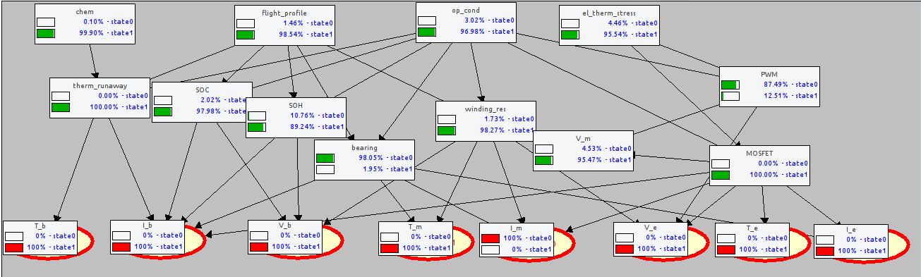
We applied this framework to the powertrain BN, as shown in the schematic of Fig. 7. In our evaluation, the sensor nodes are observable and clamped to their current values. The resulting posterior probabilities of the other nodes are then calculated. For instance, in the scenario depicted, all sensor readings are nominal except for an abnormal motor current, . The BN correctly infers a high posterior probability for the “bad motor bearing” fault mode, identifying it as the likely root cause. It is important to note that this specific example does not incorporate temporal monitors.
3.5 Defining Temporal Monitors
R2U2 monitors are used in our architecture to pre-process sensor signals (e.g., by thresholding) and to watch conditions in sensor signals and outputs of the BN over time. In order to allow simple signal processing, the input language for R2U2 can, in addition to Boolean Variables, contain arithmetic expressions, like .
For diagnostic purposes, there exist a number of different kinds of monitor patterns, including (see also Table 3):
- Thresholding:
-
such monitors perform simple signal processing tasks and determine if the current signal value is above or below a certain threshold, or is within a given range.
- Persistency:
-
a condition is considered to be persistent if it is consecutively true for at least time steps: . Such formulas are used to filter out short dropout or nuisance signals.
- Conditions:
-
failure conditions might be only considered, when certain conditions hold, e.g., when the system is in a specific mode.
- Transient blocking:
-
upon a change in the system (e.g., a mode change), a failure condition is blocked during a certain temporal interval
- Occurrence:
-
these types of monitors can determine if a signal or event occurs more than times within a given interval. This type of monitors can be used to trigger events based upon failure rates, e.g., there should not be more than 3 ill-formed data packets within a 10s interval.
- Expectations:
-
these kinds of formulas can be used to monitor if certain events occur before, during, or after a certain triggering event or condition. E.g., after touchdown, the engine RPM should be within 30 seconds below 10.
Each of the variables of these formulas can be Boolean’s obtained by thresholding sensor signals or the posterior probabilities of the failure-mode nodes of the diagnostic BN. This capability allows use to write monitors, which depend on diagnoses. E.g., if the health of a lidar sensor has been poor for at least the last minute, then only large measurement errors causes the triggering of a failure mode. Such formulas can be used to customize the diagnosis system based upon current diagnostic results and health status. If a subsystem has been diagnosed with a poor health, it might be necessary to tolerate larger error margins in order to avoid cascading of failure conditions.
| Formula | L | description |
|---|---|---|
| PT | battery low voltage test succeeds, if the battery voltage is lower than 12V continuously for at least the last minute | |
| FT | when motor is started, we expect an increase in RPM of at least 100 within the next 10 seconds | |
| PT | the motor should not be overly hot for a longer period of time except when in strong climb mode | |
| FT | the battery is not overheated and within the next 10 minutes, the battery voltage shall not fall below 12V | |
| PT | The LIDAR sensor is diagnosed as bad, if it had poor health for more than one consecutive minute | |
| PT | the battery voltage has been low for the last 10 minutes and the LIDAR sensor is unhealthy |
3.5.1 Synchronous Observers
Besides the (asynchronous) temporal observers described in Section 3.5 for past time and future time linear temporal logic, R2U2 also provides synchronous observers for future time logic. Whereas the observers for ptLTL can be valuated at each point in time, future-time observers might need to be valuated at a later time, because R2U2 cannot look into the future. For example, the ftLTL formula cannot be valuated at the beginning of the interval, because it is not yet known if will become true within the next 10 seconds. Thus, this formula can, in the worst case, only valuated after 10 seconds. R2U2 provides that information, but the use of ftLTL formulas for monitoring is not suitable for our application.
In contrast, synchronous observers can be valuated at each point in time. Introduced in [24], they return one of three possible values: false, maybe, true. Their highly efficient implementation in R2U2 makes them an ideal candidate for temporal monitors. In addition, the three-values logic values can be directly carried over to the diagnostic Bayesian network. Here, the observable sensor nodes now get a third state labeled “maybe”.
Its usefulness for diagnostic reasoning with synchronous future temporal monitors becomes evident when we look at the following example. Encoding a monitor for “the UAV shall reach an altitude of 300ft within 20 seconds if the ESC status is OK” as
provides valuable information at any point in time. Whereas the asynchronous observer can only valuated after 20 seconds, the synchronous observer returns “maybe” even at the beginning of the interval, indicating that the UAV can still reach the required altitude. Only in the case, the ESC is not working, or the 20 second interval has passed, “false” is returned. This additional piece of instantaneous information can be used to improve the diagnosis and can also support autonomous decision-making: in the “maybe”-case, the flight might be continued if the additional risk can be justified, whereas the “false” will need to cause an abortion of the mission right away.
3.6 Practical Example
We illustrate our approach with a simple model of an electric powertrain for a UAS system. As shown in Figure 8A, the system consists of a li-ion battery , the brushless dc motor (only one shown here), and the electronic speed control . For each of the components, we measure temperature , voltage and current . In the high-fidelity simulator, which uses physical and electro-chemical models, measurements are obtained in 10 second intervals. Figure 8B shows the measurement signals which are typical for a nominal situation, where between and the motor load is increased, leading to increased currents and a slight rise in battery temperature. The battery voltage slowly decreases as the battery discharges as load decreases based on operational modes. Toward the end of the scenario, the battery is near-empty and discharges very quickly.
In the nominal scenario, voltages and currents at each component are the same. As shown in Figure 5, our diagnostic BN has input nodes for temperatures, currents, and voltages, and is capable of diagnosing battery-related issues (thermal runaway, low state-of-charge, low state-of-health),, motor issues (bearing problems and change in the resistance of the motor winding), as well as in the electronic controller (power MOSFET electronics, or pulse-width-modulation (PWM) issues).
A B
Figure 9 shows the original nominal signals for the battery, their discretizations with R2U2, as well as the posterior probabilities for the SOC and SOH nodes. Most significantly, a is considered low battery voltage (V_batt_low) and V_batt_nom is a battery voltage between 20V and 26V. The figure shows that with lower voltage through increased load, and through discharge, the BN nodes for SOC and SOH change, indicating a low state of charge. Toward the end of the scenario, the battery is drained and the voltage goes off-nominal. For this scenario, a simple BN is sufficient and no temporal operators are necessary. In the next scenario, however, we need to deal with noisy signals: the battery voltage signal can have drop-outs of up to 30 seconds. These dropouts, however, should not count toward a highly discharged battery. In our framework, we subject the battery voltage signal to the R2U2 formula
The noise in Figure 9 has been eliminated properly. If we want to filter out longer-lasting periods of low voltage, like the time between and in Figure 8B, the R2U2 formula just needs to be adjusted; the additional memory overhead for processing the temporal formula is minimal (just a ring buffer for 90 integer variables). This is in stark contrast to using a dynamic BN, which would require to replicate the basic network 90 times.
A B
Figure 10 illustrates a diagnostic scenario in which the order of events is important. Initially, a flight is operating under nominal conditions. After some time, the motor current () begins to increase while the voltage () stays constant. In response, the Bayesian Network (BN) diagnoses a potential issue with the motor’s bearing or winding. The resulting increase in friction and current then causes the motor temperature () to rise. Once surpasses a critical threshold, the posterior probability for both “bearing” and “winding” failures becomes very high. This clearly points to a motor malfunction, but a static BN that fails to consider the sequence of events cannot differentiate between these two failure modes, leading to an ambiguous diagnosis.
In our framework, we add a past-time temporal formula to the output of the BN:
A B
Only if an issue with the motor bearing has been flagged continuously for at least 100s and then, within 10 seconds, the bearing and the winding issues are flagged at the same time for at least 20 seconds, we can disambiguate the situation and infer that the bearing issue is the root cause. The 10 second grace time of the temporal “S” (Since) operator is used to minimize transient effects observed due to change in operational modes.
The symmetric R2U2 formula for the winding issue would look like:
Figure 10 shows traces for both scenarios. Although a single DBN would be capable of modeling this situation, the complex temporal dependencies would require a large and complex DBN.
4 Related Work
Previous work has extensively utilized dynamic Bayesian networks (DBNs) for system diagnosis and reliability assessment. Addressing the shortcomings of traditional model-based approaches, Lerner et al. [15] proposed using a temporal causal graph (TCG) to structure a DBN for representing dynamic variable relationships. This DBN framework has been applied to several domains. In the field of reliability engineering, Lewis et al. [16] demonstrated the use of DBNs for risk assessment and highlighted the importance of modeling the health state of complex systems. Other related research includes the work of Arocha et al. [1], who developed a method for identifying reasoning strategies in medical applications through cognitive-semantic analysis.
In contrast to our approach, which prioritizes network size and efficiency, the methodology presented by Cai et al [4]. illustrates the trade-offs inherent in using Dynamic Bayesian Networks (DBNs). Their work effectively addresses the challenge of diagnosing complex temporal faults – including transient, intermittent, and permanent failures – by explicitly modeling a system’s dynamic degradation over time. To achieve this, their DBN employs Markov chains, which replicate the network structure across multiple time slices. While this allows them to classify fault types based on evolving posterior probabilities, this replication is precisely what leads to significantly larger and more computationally intensive models – a complexity our architecture is designed to avoid.
5 Conclusions
In this paper, we have introduced a powerful diagnostic system that successfully untangles temporal dynamics from probabilistic reasoning. Our key innovation – decoupling the R2U2 temporal monitoring engine from a static Bayesian Network (BN) – offers the best of both worlds: highly efficient evaluation of complex temporal conditions without the exponential complexity and network replication inherent in traditional Dynamic BNs. This ensures the core diagnostic model remains compact, transparent, and easy to maintain.
Looking ahead, our work will focus on making the developed methodology more accessible and robust for additional complex systems. The most critical next step is to streamline the modeling process itself. We will achieve this by integrating FRET, an open-source tool that automatically translates requirements written in structured natural language to formal temporal logic. This will dramatically accelerate development and eliminate the error-prone task of manual formula definition. Simultaneously, we will refine the automated generation of the Bayesian Network, deepening its integration with industry-standard modeling and analysis tools to create a seamless, end-to-end diagnostic framework.
References
- [1] Jose F Arocha, Dongwen Wang, and Vimla L Patel. Identifying reasoning strategies in medical decision making: a methodological guide. Journal of biomedical informatics, 38(2):154–171, 2005. doi:10.1016/J.JBI.2005.02.001.
- [2] A Bobbio, L Portinale, M Minichino, and E. Ciancamerla. Improving the analysis of dependable systems by mappping fault trees into bayesian networks. In Reliability Engineering and Systems Safety, volume 71, pages 249–260, 2001. doi:10.1016/S0951-8320(00)00077-6.
- [3] Borzoo Bonakdarpour and Scott A. Smolka, editors. Runtime Verification - 5th International Conference, RV 2014, Toronto, ON, Canada, September 22-25, 2014. Proceedings, volume 8734 of Lecture Notes in Computer Science. Springer, 2014. doi:10.1007/978-3-319-11164-3.
- [4] Baoping Cai, Yu Liu, and Min Xie. A dynamic-bayesian-network-based fault diagnosis methodology considering transient and intermittent faults. IEEE Transactions on Automation Science and Engineering, 14(1):276–285, 2016. doi:10.1109/TASE.2016.2574875.
- [5] Mark Chavira and Adnan Darwiche. Compiling Bayesian networks using variable elimination. In IJCAI, pages 2443–2449. Morgan Kaufmann Publishers Inc., 2007. URL: http://ijcai.org/Proceedings/07/Papers/393.pdf.
- [6] A. Darwiche. SamIam: Sensitivity analysis, modeling, inference, and more. URL: http://reasoning.cs.ucla.edu/samiam/.
- [7] A. Darwiche. Modeling and reasoning with bayesian networks. In Modeling and Reasoning with Bayesian Networks, 2009.
- [8] Adnan Darwiche. Recursive conditioning. Artificial Intelligence, 126(1-2):5–41, 2001. doi:10.1016/S0004-3702(00)00069-2.
- [9] Adnan Darwiche. A differential approach to inference in Bayesian networks. J. ACM, 50(3):280–305, 2003. doi:10.1145/765568.765570.
- [10] Johannes Geist, Kristin Y. Rozier, and Johann Schumann. Runtime observer pairs and bayesian network reasoners on-board FPGAs: Flight-certifiable system health management for embedded systems. In Runtime Verification - 5th International Conference, RV 2014, Toronto, ON, Canada, September 22-25, 2014. Proceedings, pages 215–230, 2014. doi:10.1007/978-3-319-11164-3_18.
- [11] Alvaro García Eduardo Gilabert. Mapping fmea into bayesian networks. International Journal of Performability Engineering, 7(6):525–537, 2011.
- [12] F. V. Jensen, S. L. Lauritzen, and K. G. Olesen. Bayesian updating in causal probabilistic network by local computations. Computational Statistics, Quarterly 4:269–282, 1990.
- [13] Ron Koymans. Specifying real-time properties with Metric Temporal Logic. Real-time systems, 2(4):255–299, 1990. doi:10.1007/BF01995674.
- [14] S. L. Lauritzen and D. J. Spiegelhalter. Local computations with probabilities on graphical structures and their application to expert systems. Journal of the Royal Statistical Society, 50(2):157–224, 1988.
- [15] U. Lerner, R. Parr, D. Koller, and G. Biswas. Bayesian fault detection and diagnosis in dynamic systems. In Proc. of the Seventeenth national Conference on Artificial Intelligence (AAAI-00), pages 531–537, 2000. URL: citeseer.ist.psu.edu/lerner00bayesian.html.
- [16] Austin D Lewis and Katrina M Groth. A dynamic bayesian network structure for joint diagnostics and prognostics of complex engineering systems. Algorithms, 13(3):64, 2020. doi:10.3390/A13030064.
- [17] Zhaoyu Li and Bruce D’Ambrosio. Efficient inference in bayes networks as a combinatorial optimization problem. International Journal of Approximate Reasoning, 11(1):55–81, 1994. doi:10.1016/0888-613X(94)90019-1.
- [18] O. J. Mengshoel. Designing resource-bounded reasoners using Bayesian networks: System health monitoring and diagnosis. In DX, pages 330–337, 2007.
- [19] Ole J. Mengshoel, Dan Roth, and David C. Wilkins. Portfolios in stochastic local search: Efficiently computing most probable explanations in Bayesian networks. J. Autom. Reason., 46(2):103–160, 2011. doi:10.1007/S10817-010-9170-5.
- [20] D.J. Musliner, J.A. Hendler, A.K. Agrawala, E.H. Durfee, J.K. Strosnider, and C. J. Paul. The challenges of real-time AI. Computer, 28(1):58–66, 1995.
- [21] James D. Park and Adnan Darwiche. Complexity results and approximation strategies for map explanations. J. Artif. Int. Res., 21(1):101–133, 2004. doi:10.1613/JAIR.1236.
- [22] J. Pearl. Bayesian networks: A model cf self-activated memory for evidential reasoning. In 7th Conference of the Cognitive Science Society, 1985.
- [23] J. Pearl. Causality: models, reasoning and inference. MIT Press Cambridge, MA, 2000.
- [24] Thomas Reinbacher, Jörg Brauer, Martin Horauer, Andreas Steininger, and Stefan Kowalewski. Runtime verification of microcontroller binary code. Sci. Comput. Program., 80:109–129, February 2014. doi:10.1016/j.scico.2012.10.015.
- [25] Thomas Reinbacher, Kristin Yvonne Rozier, and Johann Schumann. Temporal-logic based runtime observer pairs for system health management of real-time systems. In Erika Ábrahám and Klaus Havelund, editors, Tools and Algorithms for the Construction and Analysis of Systems - 20th International Conference, TACAS 2014, Held as Part of the European Joint Conferences on Theory and Practice of Software, ETAPS 2014, Grenoble, France, April 5-13, 2014. Proceedings, volume 8413 of Lecture Notes in Computer Science, pages 357–372. Springer, 2014. doi:10.1007/978-3-642-54862-8_24.
- [26] Johann Schumann, Nagabhushan Mahadevan, Adam Sweet, Anupa R. Bajwa, Michael Lowry, and Gabor Karsai. Model-based System Health Management and Contingency Planning for Autonomous UAS. In AIAA Scitech Forum, 2019. URL: https://arc.aiaa.org/doi/pdf/10.2514/6.2019-1961.
- [27] Johann Schumann, Kristin Y. Rozier, Thomas Reinbacher, Ole J. Mengshoel, Timmy Mbaya, and Corey Ippolito. Towards real-time, on-board, hardware-supported sensor and software health management for unmanned aerial systems. In Proceedings of the 2013 Annual Conference of the Prognostics and Health Management Society (PHM2013), October 2013.
- [28] Johann Schumann, Kristin Y. Rozier, Thomas Reinbacher, Ole J. Mengshoel, Timmy Mbaya, and Corey Ippolito. Towards real-time, on-board, hardware-supported sensor and software health management for unmanned aerial systems. International Journal of Prognostics and Health Management, 6(21):1–27, 2015.
- [29] Prakash P. Shenoy. A valuation-based language for expert systems. International Journal of Approximate Reasoning, 3(5):383–411, 1989. doi:10.1016/0888-613X(89)90009-1.
- [30] Nevin Zhang and David Poole. A simple approach to Bayesian network computations. In Proceedings of the Tenth Canadian Conference on Artificial Intelligence, pages 171–178. Morgan Kaufmann, 1994.