Data-Driven Fault Detection and Isolation Enhanced with System Structural Relationships

Abstract
Fault detection and isolation are becoming increasingly important as modern systems become more complex. To encourage the development of new fault detection solutions that can operate with limited noisy data and an incomplete mathematical model, the DX 2025 LiU-ICE competition for diagnosis of the air path of an internal combustion engine was introduced. In this paper, we present our winning solution to this competition. Our fault detection architecture starts with a semi-supervised Transformer Autoencoder trained to reconstruct nominal data. Detected faults are then passed through a rule-based fault persistence filter that aims to suppress false positives. Once a fault is detected, we use four neural networks trained to estimate features determined from structural analysis of a partial system model. The residuals of these networks are fed to a supervised fault classification network that estimates the fault probabilities. With this architecture, we achieved an 87% detection rate with a 0% false alarm rate on the provided competition data. Additionally, our isolation architecture assigned the correct fault 73.8% probabilty on average. On unseen competition data from a new driving cycle, we achieved a 100% detection rate and assigned the correct fault 66.2% probability on average. On the other hand, the Transformer Autoencoder failed to transfer to the new driving conditions, causing many false alarms. We discuss ways future work can reduce this.
Keywords and phrases:
fault detection, fault isolation, autoencoderCategory:
DX CompetitionCopyright and License:
2012 ACM Subject Classification:
Computing methodologies Anomaly detection ; Applied computing Engineering ; Computing methodologies Neural networksFunding:
This material is based upon work supported by the National Science Foundation Graduate Research Fellowship Program under Grant No. 2444112. Any opinions, findings, and conclusions or recommendations expressed in this material are those of the author(s) and do not necessarily reflect the views of the National Science Foundation.Editors:
Marcos Quinones-Grueiro, Gautam Biswas, and Ingo PillSeries and Publisher:
1 Introduction
Modern systems, such as those in transportation, manufacturing, and energy, are becoming increasingly complex and critical to daily life. As the complexity of these systems increases, the number of potential faults often increases. These faults can lead to performance degradation, safety risks, or even catastrophic failure [9]. Therefore, fault detection and isolation (FDI) methods are essential to ensure the reliability, efficiency [5], and safety [26] of complex systems.
Traditional FDI approaches are model-based, developing system-specific methods [1]. Model-based methods have historically relied on analyzing the patterns of the difference between observed sensor values and the output predicted by a mathematical model of the system, known as residuals [10]. This framework serves as the foundation for many modern model-based approaches, such as [25, 6]. Although model-based methods can be successful in detecting and isolating faults, they are limited in scenarios without an accurate and complete model of the system. In these scenarios, data-driven models can be applied if behavioral data has been collected for the system. Data-driven fault detection and diagnosis methods can be classified as supervised or unsupervised [1]. Supervised approaches leverage labeled training data to discriminate between faulty and nominal data or to classify the fault category, e.g., [24]. In many domains, obtaining labeled fault data is infeasible or prohibitively expensive. In these cases, unsupervised or semi-supervised data-driven approaches have been used requiring partially or no labeled data , e.g, [4]. While data-driven FDI approaches offer promising solutions when a complete system model is unavailable, they can be combined with model-based approaches when some knowledge of the system is available, such as in [22]. Despite the increasing number of FDI solutions, inaccuracies in the system model, limited training data, and measurement noise complicate the task, and existing solutions do not fully address these issues [14].
With these challenges in mind, the LiU-ICE benchmark was introduced as a DX 2025 competition [14]. This benchmark focuses on fault detection and isolation of the air path of an internal combustion engine. It consists of an analytical model with unknown parameters and data from nominal and four faulty scenarios with varying magnitudes. In this paper, we present a solution to the LiU-ICE DX 2025 competition. Our solution consists of two steps: fault detection and isolation. To detect faults, we use a semi-supervised Transformer Autoencoder that aims to reconstruct the current data sample given a window of recent samples. When the reconstruction error is higher than a threshold determined from nominal data, the sample is flagged as a potential fault. Potential faults are filtered by a rule-based persistence filter designed to suppress false alarms. After detection, we isolate faults. Using structural analysis, we obtain Minimally Structurally Over-determined (MSO) sets. For each MSO set, we train a feature estimation neural network that learns system relationships. The residuals of each feature estimation network are fed to a supervised fault classifier that estimates the probabilities of each fault.
The contributions of this paper are as follows.
-
We present a data-driven fault detection and isolation architecture enhanced with system structural relationships that achieved first place in the LiU-ICE DX 2025 competition.
-
We perform an in-depth analysis of the strengths and limitations of our approach on the provided competition data. On the evaluation data, we discuss the performance, including autoencoder transfer issues that cause a high false alarm rate and potential solutions.
The remainder of the paper is structured as follows. In Section 2, we give necessary background about the competition, dataset, and performance metrics. In Section 3, we describe our fault detection and isolation architecture. In Section 4.2, we describe the results on the provided competition data and unseen evaluation data. In Section 5, we discuss transfer issues on the unseen competition data and how future work can resolve this problem. Finally, in Section 6, we conclude the paper.
2 Competition and Dataset Preliminaries
This paper describes a solution to the 2025 International Conference on Principles of Diagnosis and Resilient Systems (DX’25) LiU-ICE industrial fault diagnosis benchmark competition [14] first described in [17]. This competition calls for the development of a diagnosis system for the air path of an internal combustion engine.
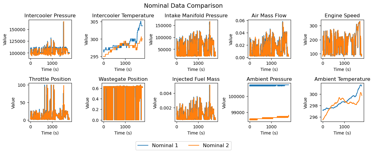
The data consists of ten signals measured on a real engine test bed at 20Hz. The ten signals consist of eight sensor signals: the intercooler pressure, intercooler temperature, intake manifold pressure, mass flow through the air filter, throttle actuator position, engine speed, ambient pressure, and ambient temperature. There are also two actuator signals: the requested injected fuel mass and the requested wastegate actuator position. Of these, we removed the ambient pressure, ambient temperature, and intercooler temperature, as they were difficult to reconstruct and led to worse fault detection performance. Figure 1 shows the ten available signals on two nominal driving cycles. The intercooler temperature, ambient pressure, and ambient temperature are different despite both being from nominal driving cycles, further justifying their removal as a preprocessing step.
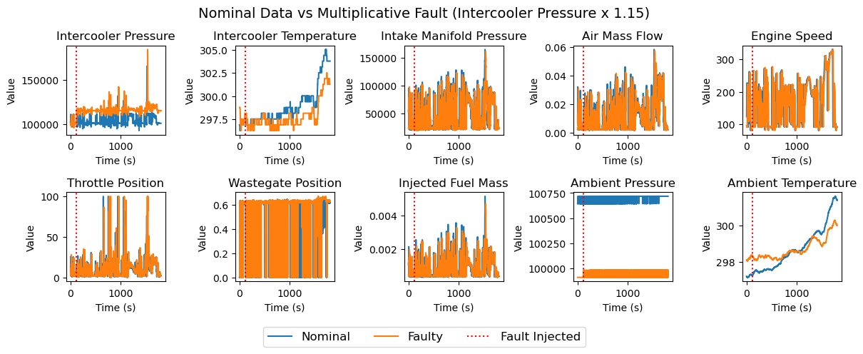
In this challenge, there are four faults of varying magnitudes. There are three sensor faults and one leakage fault. The three sensor faults are multiplicative faults in the sensors measuring the air mass flow (WAF), intercooler pressure (PIC), and intake manifold pressure (PIM). These were introduced by multiplying the sensor measurement by a constant value of 0.8, 0.85, 0.9, 0.95, 1.05, 1.1, or 1.15 for the remaining duration of the driving cycle. An example showing the PIC fault multiplied by 1.15 (denoted PIC 115 in the dataset) is shown in Figure 2. After the fault was introduced around 120 seconds into the driving cycle, the intercooler pressure sensor measurement increased. The leakage fault was in the intake manifold (IML). A 4mm or 6mm leak was introduced by opening a valve.
The dataset for the competition consists of 25 driving cycles, 1 for each magnitude of sensor fault (7 per fault), 1 for each of the two magnitudes of leakage fault, and 2 nominal trajectories. In the faulty datasets, the fault was introduced around 120 seconds into the cycle and persists until the end of the trajectory. For our experiments, we split the data into sub-datasets used for different tasks in the remainder of the paper. These are as follows.
-
Nominal Dataset: the two full nominal trajectories representing the nominal state of the system. This was used for training most models.
-
Validation Dataset: the full trajectories (nominal and faulty data) for the 4mm IML, 080 PIC, 090 PIC, 095 PIC, 105 PIC, 115 PIC, 085 PIM, 090 PIM, 095 PIM, 110 PIM, 115 PIM, 080 WAF, 090 WAF, 095 WAF, 105 WAF, and 115 WAF faults. This totals 16/23 faulty trajectories. This was used for calibrating parameters, calibrating hyperparameters, and evaluating performance while developing our methodology.
-
Testing Dataset: the full trajectories (nominal and faulty data) for the 6mm IML, 085 PIC, 110 PIC, 080 PIM, 105 PIM, 085 WAF, and 110 WAF faults. This totals 7/23 faulty trajectories. This was used for the evaluation of the generalization performance of our methodology to new fault magnitudes.
-
Full Faulty Dataset: the full trajectories (nominal and faulty data) of all 23 fault magnitudes. This was used for the full evaluation of the methodology.
The competition is scored using three evaluation metrics, defined as follows.
-
False Alarm Rate (FAR): the percentage of faults detected when there is no fault in the system.
-
True Detection Rate (TDR): the percentage of faults detected when there is a fault in the system.
-
Fault Isolation Accuracy (FIA): the average probability given to the actual fault when a fault is correctly detected. Note that this is not the fault classification accuracy.
The final score is determined by averaging the three evaluation metrics above (taking 1-FAR instead of the FAR).
3 Method
In this Section, we detail our unsupervised data-driven fault detection and supervised fault isolation methodology. We include details about the general methodology, model training process, and hyperparameter tuning process.
3.1 Fault Detection
First, we perform fault detection. Our fault detection architecture, shown in Figure 3, consists of an autoencoding step to obtain an initial unsupervised fault label and a rule-based filtering step to reduce false positives caused by noisy samples.
3.1.1 Transformer Autoencoder
To detect faults, we train a Transformer Autoencoder model on the nominal training trajectories. Autoencoder models are commonly used for unsupervised anomaly detection [20]. Autoencoders compress data to a lower dimensional space then reconstruct the original data from the lower-dimensional representation. By learning this task on nominal data in a semi-supervised way, an autoencoder can learn a representation of the nominal behavior of the system. It operates on the key assumption that the it will not generalize to unseen data distributions and will therefore only reconstruct nominal data well. Then, if anomalous (likely faulty) data is fed to the autoencoder, it will reconstruct it poorly. A threshold can be set on the reconstruction error to assign binary fault detection classifications.
More formally, we have an encoder neural network where is the space of the measured data and is the space of compressed representations and . We also have a decoder neural network that reconstructs the input data. Then, the autoencoder operation can be formulated as follows
| (1) |
where is an input sample and is its reconstruction. An autoencoder is typically trained to minimize the reconstruction error on nominal data, quantified using the mean-squared error loss as follows
| (2) |
To determine whether the input is faulty, its reconstruction error can be compared against a threshold determined by applying the autoencoder to nominal data, i.e., it is faulty if .
The autoencoder framework allows for freedom in choosing the encoder and decoder networks. For the system studied in this paper, we use Transformer neural networks. Transformers [21] are sequence-based neural networks that use self-attention mechanisms instead of recurrence. Self-attention allows each data point in the sequence to update its representation using every other point in the sequence in parallel. Using this mechanism Transformers have been shown to outperform Recurrent neural network-based approaches in time series domains like speech [15]. By using a powerful sequential model like a Transformer as the encoder and decoder of the autoencoder, we can learn potential temporal relationships in the data and leverage them for fault detection. The architecture of this model, taking a window of inputs and reconstructing the current input, is shown at the top of Figure 3.
As the Transformer Autoencoder model is the first step in our fault detection and isolation pipeline, it is important that it is properly calibrated. To do so, we started by tuning the hyperparameters. We tuned the hyperparameters using the Tree-Structured Parzen Estimator algorithm [3] included in Optuna [2], allowing for an intelligent optimization of both discrete and continuous hyperparameters. We optimized the hyperparameters that maximized the detection score, a modification of the competition score from Section 2 and quantified as follows
| (3) |
where TDR is the true detection rate and FAR is the false alarm rate. This score measures the balance of true fault detections and false alarms. During hyperparameter optimization, the Transformer Autoencoder was trained on the two full nominal trajectories. Data was normalized between 0 and 1 using the minimums and maximums of the training data. An initial threshold vector was chosen as the maximum reconstruction error for each feature across the training sets after convergence. We evaluated the detection score on the 16 validation trajectories, described in Section 2. The optimal hyperparameters after 100 trials are shown in Table 1.
| Batch Size | Latent Dim. | Trans. Dim. | Feedforward Dim. | Thresh. | Dropout % |
|---|---|---|---|---|---|
| 128 | 4 | 32 | 128 | -0.02 | 28.1 |
| Learn. Rate | Num. Epochs | Num. Heads | Num. Layers | Sequence Len. | - |
| 0.003 | 8 | 2 | 3 | 5 |
From Table 1, we can see that the threshold, a modification of the reconstruction error threshold chosen as the maximum nominal reconstruction error for each feature, was chosen to be . To maximize the Detection Score, the hyperparameter optimization decreased the threshold, allowing some false positives. Since this hyperparameter controls the tradeoff between true positive and false positive rate, we performed an additional hyperparameter search over the threshold for each feature independently. This led to the following thresholds. Intercooler pressure , intercooler temperature , intake manifold pressure , air mass flow , engine speed , throttle position , and injected fuel mass . With different thresholds and thresholds for each, the detection does not have to be sensitive to any one reconstructed feature.
3.1.2 Fault Persistence Filter
While the Transformer Autoencoder trained with optimized hyperparameters detects faults reasonably well (Detection Score on validation data), it is sensitive to noise in the data, causing false positives. Additionally, it may miss some detections after the fault occurs. To address this issue, we develop a rule-based fault filtering approach. This approach assumes that once a fault is introduced, it will persist until the end of the trajectory. In other words, there are no intermittent faults.
The rule-based fault persistence filtering, shown in the bottom block of Figure 3, keeps track of the fault detection predictions by the Transformer Autoencoder. If of the last predictions are a (there is a fault), then the filter deems the system faulty and outputs 1 for the remainder of the trajectory. Otherwise, the system is not considered faulty, so the filter outputs 0. More formally, assume the detections are being tracked in a boolean queue , filled with 0s at the start of each trajectory, and is the state of the queue at time . Then, the filtering logic is as follows
| (4) |
We tuned the parameters and manually on the validation set using the Transformer Autoencoder model trained with optimized hyperparameters. We found that and (7 seconds) worked best.
3.2 Fault Isolation
Once a fault is persistently detected, we isolate the fault. Our fault isolation architecture, shown in Figure 4, consists of two phases. First, we train neural networks that perform a semi-supervised feature estimation based on relationships determined from structural analysis of the provided partial model. Then, we classify the fault probabilities using a supervised fault classification neural network that takes the feature estimation model errors as input to use the system structure information for fault isolation.
3.2.1 Data-Driven Residual Generation Through Structural Analysis
To isolate faults, we first determine relationships between features by performing a structural analysis of the partial system model provided in the competition.
Structural analysis defines a set of methods that allow to characterize the analytical redundancy in a system that can be exploited for fault detection and diagnosis. Obtaining data-driven residuals through structural analysis begins with defining the analytical model of the dynamic system that describes the underlying physics that drive the system’s behavior, typically through differential algebraic equations. A structural model is represented as a bipartite graph or a logical/incidence matrix that describes the qualitative relationship between model equations and variables [13]. The Dulmage-Mendelsohn decomposition is applied to the structural model to partition it into under-determined, exactly determined, and over-determined parts. The over-determined part contains analytical redundancy – meaning there are more equations than unknown variables.
Within the over-determined part of the model, structural analysis methods identify redundant equation sets. Of particular interest are the Minimally Structurally Over-determined (MSO) sets. MSO sets represent the minimal redundant equation sets that can be used for residual generation, corresponding to the smallest parts of the system that can be monitored separately [17, 18]. From these MSO sets, computational graphs are derived by designating one equation as the residual and establishing a causal computation sequence for other variables from known signals. In Figure 4, the green boxes in the MSO matrix indicate the variable that can be represented using the other (blue) known signals. This derived structure is used to design a data-driven model, where non-linear functions and dynamic states from the computational graph are mapped to components like Multi-layer Perceptrons (MLPs) within the network [13, 17, 18]. These models are intentionally designed to resemble the physical system’s structure, embedding physical insights into the data-driven approach. These models are then trained exclusively on nominal (fault-free) data to accurately learn the system’s expected behavior under normal conditions. Training aims to minimize the model’s prediction error for a target signal.
Finally, the data-driven residual is generated by calculating the difference between the actual measured value of the target signal and the output predicted by the trained data-driven model. This process results in residuals that act as anomaly detectors, highlighting deviations from expected nominal behavior, which is particularly useful when data from faulty scenarios is limited.
3.2.2 MLP Feature Estimators
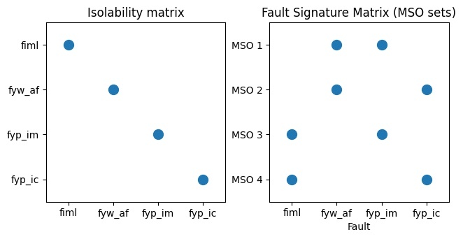
Based on the MSO matrix, we use a simple test selection strategy that finds sets of tests that, ideally, fulfills specified isolability performance specifications [16]. For each MSO in the set , we can use the system relationships to generate feature estimator models. According to the structural analysis, these four can be used to isolate any of the known faults, in theory (see Figure 5 for the isolability matrix and fault signature matrix). As shown at the top of Figure 4, we train one multi-layer perceptron neural network model for each row in the MSO matrix. These estimate the target feature using the predictor features and are small, 2-layer 64-neuron networks. The hyperparameters of these networks were empirically determined and kept fixed. They are trained using the mean-squared error. These models can be used to isolate a fault by checking whether their estimation error is above a threshold. When this happens, we say a model “triggers”. This can be expressed for a model as follows,
| (5) |
where are the predictive features, is the target feature, and is some threshold. By comparing to the threshold, we can quantify the model’s absolute estimation error. In the future, we will explore more advanced architectures like grey-box Recurrent Neural Networks [13] or Neural Ordinary Differential Equations [18].
3.2.3 Fault Classification
With the trained feature estimators for each MSO set, we can theoretically isolate faults. See Figure 5; all faults are isolable. To isolate the IML fault (column 1 of the rightmost plot), for example, we can check whether the feature estimators for MSO 3 and 4 trigger while the other two do not. The other faults could be isolated following the same pattern.
We could isolate faults with moderate success following this method. However, the reality of the noisy, limited data made consistently isolating all faults impossible, even with added rule-based filtering and threshold tuning. To address this issue, we leveraged the labeled faulty data to train a supervised fault classifier.
The fault classifier, as shown at the bottom of Figure 4, replaces the error thresholding and fault signature matrix lookup with a neural network. This allows us to represent complex relationships between the feature estimation errors while maintaining the structure of the MSO set models. The classifier takes the feature estimation error as input and outputs the softmax probabilities of each of the four fault types. We trained this model on all available anomalous data to ensure it was accurate on all fault magnitudes. During training, the weights of the feature estimators are frozen. We found that training this fault classifier allows to better characterize the feature residual space than thresholding techniques or statistical tests like CUSUM.
In evaluation mode, we process the softmax probabilities of the classifier to fit the competition format. First, we check whether the fault is unknown. If none of the four fault types has a softmax probability above 0.35, determined by analyzing the average probabilities across the anomalous data, we classify the fault as unknown. Otherwise, we classify the fault as the fault with maximum probability. We isolate these faults with 100% confidence for the competition, as the scoring encourages confident results.
4 Results
To asses our approach, we evaluated the fault detection and fault isolation components on two sets of data. The first was the data given for the competition. The second was an unseen dataset used to evaluate competition submissions.
4.1 Results on Competition Data
Using the labeled faulty and nominal data from the competition, we evaluated both the fault detection and isolation performance of our model using the competition’s evaluation metrics defined in Section 2.
4.1.1 Fault Detection
| Type | Magnitude | TDR | FAR | Detection Score |
|---|---|---|---|---|
| IML | 4mm | 0.14 | 0.00 | 0.57 |
| IML | 6mm | 0.95 | 0.00 | 0.98 |
| PIC | 080 | 0.96 | 0.00 | 0.98 |
| PIC | 085 | 1.00 | 0.00 | 1.00 |
| PIC | 090 | 1.00 | 0.00 | 1.00 |
| PIC | 095 | 1.00 | 0.00 | 1.00 |
| PIC | 105 | 1.00 | 0.00 | 1.00 |
| PIC | 110 | 0.99 | 0.00 | 1.00 |
| PIC | 115 | 1.00 | 0.00 | 1.00 |
| PIM | 080 | 0.97 | 0.00 | 0.99 |
| PIM | 085 | 0.97 | 0.00 | 0.99 |
| PIM | 090 | 0.95 | 0.00 | 0.97 |
| PIM | 095 | 0.94 | 0.00 | 0.97 |
| PIM | 105 | 0.61 | 0.00 | 0.81 |
| PIM | 110 | 0.62 | 0.00 | 0.81 |
| PIM | 115 | 0.92 | 0.00 | 0.96 |
| WAF | 080 | 0.98 | 0.00 | 0.99 |
| WAF | 085 | 0.85 | 0.00 | 0.93 |
| WAF | 090 | 0.46 | 0.00 | 0.73 |
| WAF | 095 | 0.91 | 0.00 | 0.96 |
| WAF | 105 | 0.85 | 0.00 | 0.93 |
| WAF | 110 | 0.94 | 0.00 | 0.97 |
| WAF | 115 | 0.98 | 0.00 | 0.99 |
| Average: | 0.87 | 0.00 | 0.93 | |
The results for the fault detection performance on all faulty data are shown in Table 2. This table shows the True Detection Rate (TDR), False Alarm Rate (FAR), and Detection Score (from Equation (3)) broken down by fault type and magnitude. From this, we can see that the proposed fault detection architecture detected 87% of faults with a 0% False Alarm Rate. This led to a Detection Score of 0.93. While some number of false positives may have led to a higher Detection Score, minimizing false positives is necessary for real applications.
The low FAR can be attributed to the fault persistence filter (see the bottom of Figure 3). This filter divides the current trajectory into nominal and faulty states. When 80% of the last 7 seconds have been flagged as anomalous by the Transformer Autoencoder, it considers the trajectory to be faulty. Otherwise, any detections by the autoencoder are attributed to noise or smaller anomalies and are suppressed.
While the fault persistence filter reduced the FAR, it also caused some faults to be detected late. For example, consider the 4mm IML fault, shown in Table 2. This fault was only detected during the last 14% of the faulty trajectory. Without the persistence filter, fault detections may have appeared earlier, at the cost of additional false alarms. With a more sensitive persistence filter, e.g., 50% of the last 3 seconds, this fault may have been consistently detected earlier. However, the chosen filter parameters maximized the overall Detection Score.
Next, we can analyze which fault types and magnitudes were more difficult to detect. From Table 2, we can see that the PIC faults were nearly always perfectly detected. All PIM faults where the sensor reading was reduced (magnitude ) were detected with more than 90% accuracy. When the sensor reading was increased by 5 and 10% (magnitudes 105 and 110), the detection rate dropped to around 60%. The only WAF fault detected with a rate less than 85% was when the sensor reading decreased by 10%. In this case, the fault was not detected consistently enough when it was introduced around 120 seconds into the trajectory to satisfy the persistence filter. A consistent anomalous behavior, according to the Transformer Autoencoder reconstructions, did not appear until around 54% into the trajectory. Since WAF faults of lower magnitude were consistently detected, this can likely be attributed to the driving behavior of this specific trajectory. For example, the impact of a WAF fault may not be clear during long periods of consistent driving speeds. Finally, the 4mm IML fault was detected much later than the 6mm IML fault. The smaller leak had a much more subtle impact on the system, causing it to be harder to detect and isolate.
4.1.2 Fault Isolation
| Type | Magnitude | P(PIC) | P(PIM) | P(WAF) | P(IML) | P(Unknown) |
|---|---|---|---|---|---|---|
| IML | 4mm | 0.086 | 0.193 | 0.337 | 0.336 | 0.048 |
| IML | 6mm | 0.059 | 0.245 | 0.310 | 0.347 | 0.039 |
| PIC | 080 | 0.887 | 0.026 | 0.085 | 0.001 | 0.001 |
| PIC | 085 | 0.887 | 0.036 | 0.075 | 0.001 | 0.001 |
| PIC | 090 | 0.853 | 0.029 | 0.111 | 0.002 | 0.004 |
| PIC | 095 | 0.641 | 0.093 | 0.214 | 0.019 | 0.034 |
| PIC | 105 | 0.703 | 0.071 | 0.170 | 0.026 | 0.030 |
| PIC | 110 | 0.892 | 0.033 | 0.055 | 0.008 | 0.012 |
| PIC | 115 | 0.930 | 0.021 | 0.047 | 0.001 | 0.001 |
| PIM | 080 | 0.003 | 0.927 | 0.057 | 0.011 | 0.002 |
| PIM | 085 | 0.005 | 0.853 | 0.124 | 0.014 | 0.003 |
| PIM | 090 | 0.010 | 0.821 | 0.141 | 0.022 | 0.005 |
| PIM | 095 | 0.044 | 0.573 | 0.303 | 0.044 | 0.035 |
| PIM | 105 | 0.028 | 0.396 | 0.556 | 0.011 | 0.010 |
| PIM | 110 | 0.030 | 0.740 | 0.196 | 0.022 | 0.013 |
| PIM | 115 | 0.014 | 0.813 | 0.137 | 0.029 | 0.007 |
| WAF | 080 | 0.027 | 0.213 | 0.752 | 0.005 | 0.003 |
| WAF | 085 | 0.016 | 0.119 | 0.821 | 0.025 | 0.019 |
| WAF | 090 | 0.033 | 0.154 | 0.789 | 0.011 | 0.013 |
| WAF | 095 | 0.042 | 0.213 | 0.708 | 0.020 | 0.017 |
| WAF | 105 | 0.038 | 0.181 | 0.759 | 0.011 | 0.011 |
| WAF | 110 | 0.018 | 0.213 | 0.755 | 0.005 | 0.008 |
| WAF | 115 | 0.032 | 0.142 | 0.788 | 0.023 | 0.015 |
| Fault Isolation Accuracy: | 0.738 | |||||
Next, we evaluated our fault isolation architecture on the faulty datasets. The average probabilities assigned to each fault type on each dataset are shown in Table 3. The overall Fault Isolation Accuracy (FIA), as defined by the competition description in Section 2, was 0.738. This means the true fault was assigned a 73.8% probability on average across the fault types and magnitudes.
For the sensor faults, this was higher. For example, the PIC fault, which was the most consistently detected, had an average FIA of 82.8%. On the other hand, the IML fault was not isolated with high probability. For the 4mm magnitude IML fault, the model assigned nearly equal average probabilities to the WAF and IML faults. At 6mm magnitude, the IML fault was assigned the highest probability, but still below 35% on average. This highlights the difficulty of detecting and isolating the leakage faults over the sensor faults in this system.
From Table 3, we can see that the average probability of an unknown fault was always low, below 5%. Since all this data was used for training the final fault classifier and none of the faults are unknown to the model, this is an expected and positive result. Future work should evaluate the model on new fault types to determine the effectiveness of the architecture in identifying unknown faults.
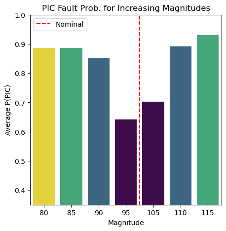

Next, we can analyze the impact of sensor fault magnitude on the isolation performance. From Table 3, we can see that the WAF fault was isolated consistently for all magnitudes. However, the PIC and PIM faults were correctly isolated with a higher average probability as the fault magnitude increased. Figure 6 shows the average probabilities assigned to these fault types as the fault magnitude increased (the sensor reading was increased or decreased by 5, 10, 15, then 20%). As the magnitudes got further away from their nominal value, which would be represented by 100, the fault was better isolated. This result is consistent with intuition, as more extreme faults should have a more dramatic impact on the system and should therefore be easier to isolate.


Since the competition metrics included in Table 3 aggregate the isolation probabilities across the driving trajectories, we cannot analyze the behavior of the fault isolation across time. To better understand this, we plotted the isolation probabilities over time for the 4mm IML fault, 10% lower magnitude WAF fault, and 15% higher magnitude PIC fault in Figure 7. Since the fault isolation architecture assigns 100% confidence in a fault when its softmax probability is above 0.35, Figure 7 shows a running average of 20 of these probabilities to show the average probability trend.
First, we can consider the most difficult fault to detect and isolate, the 4mm IML fault shown in Figure 7(a). Throughout the trajectory, this fault was consistently misidentified as the WAF and PIM faults. However, there are long periods where the IML fault is properly isolated, such as around 450s and 1000s. Even though the IML fault was not assigned the highest average probability, this consistency may lead us to classify the fault type of the trajectory as an IML fault, pointing maintainers to the intake manifold valve first.
Next, we can consider a sensor fault that was isolated well but detected poorly, the 10% lower magnitude WAF fault shown in Figure 7(b). Even though this fault was detected late, over halfway through the trajectory, the isolation algorithm consistently isolated the WAF fault with high probability before it was detected. This indicates that the impact of the fault was present in the data and that the late detection was likely due to the detection not being consistent enough early to pass the persistence filter. Additionally, when the WAF fault was not correctly isolated, it was largely classified as a PIM fault.
Finally, we can analyze the probabilities for the fault that was isolated best, the 15% higher PIC fault shown in Figure 7(c). This fault was nearly perfectly isolated and was given 100% probability for most of the trajectory.
4.2 Results on Unseen Data (Competition Results)
| Fault Type | TDR | FAR | FIA | Time (ms) |
|---|---|---|---|---|
| Nominal | – | 0.913 | – | 2.1 |
| PIC | 1.0 | 0.393 | 0.894 | 4.0 |
| PIM | 1.0 | 0.388 | 0.495 | 3.5 |
| WAF | 1.0 | 0.731 | 0.607 | 5.0 |
| Average: | 1.0 | 0.526 | 0.662 | 3.65 |
| Score: | 71.2 | |||
After the evaluation on the given competition data, the full fault detection and isolation architecture was combined and submitted. In the combined architecture, the fault isolation was only used when a fault was detected after the persistence filter. For the final competition scoring, the architecture was evaluated on data from the same fault types and magnitudes, without IML faults, generated using a different driving cycle representing city driving.
The results on this unseen data are shown in Table 4. The FAR was much higher, at 91.3% on nominal data and 73.1% on data from WAF faults. On PIC and PIM faults, the FAR was around 39%. In real applications, this many false alarms may be unacceptable. The Transformer Autoencoder needs to be recalibrated to the new distribution of nominal driving data. An in-depth discussion into why unsupervised autoencoders are so sensitive in situations like this and how to address this problem is provided in Section 5.
In terms of the other metrics, the architecture’s performance was much closer to the performance on the provided competition data. It achieved a perfect detection rate (at the expense of false alarms). It also made its predictions in less than 5 milliseconds on average, well within the data rate of 50 milliseconds. Therefore, the predictions could be used for real-time decisions. Finally, the FIA was 66.2% on average, close to the 77.6% average isolation probability for the same fault types on the training data. Overall, the final competition score was 71.2% achieving first place, with second place scoring 60.5%.
5 Discussion on Reducing Autoencoder False Alarms
While autoencoders can be very powerful for unsupervised anomaly detection, they are limited in their generalization to unseen data distributions. In a way, this is by design. Recall from Section 3 that the Transformer Autoencoder was trained to reconstruct nominal data. Then, its failure to reconstruct data from unseen distributions (anomalous data) can be used for fault detection. However, when nominal data is also out of distribution, the autoencoder may fail to reconstruct it well and classify it as faulty. This is why there was a high False Alarm Rate on the competition data generated using a different driving cycle (Section 4.2).
A simple way to reduce false alarms would be to fine-tune the autoencoder on data from the new driving cycle, ensuring it learns a more complete representation of the system’s nominal behavior, like in [11]. However, this would not permanently solve the problem, as any new out-of-distribution nominal data, such as from new driving cycles or environmental factors, might be considered anomalous. In some cases, it may be reasonable to assume the system will not encounter new nominal conditions, such as in controlled environments and testbeds. However, in many real-world applications, the environment and system usage may be nonstationary [7]. Therefore, the autoencoder must constantly adapt to new conditions.
A promising potential solution to reducing the false alarms introduced in this architecture by the Transformer Autoencoder lies in continual learning [23]. In continual learning, a model is continually adapted throughout the lifetime of its deployment. In other words, it never stops learning. This could be used to adapt the Transformer Autoencoder model to all experienced nominal conditions, reducing false alarms. This adaptation could be done online by identifying data that is assumed to be nominal or immediately after a trajectory by identifying nominal periods of data.
Aside from improving the performance of the autoencoder for fault detection on new data distributions, it could be replaced with different fault detection approaches. Many anomaly and fault detection approaches may work well and should be considered in future studies. For example, contrastive learning [12], density estimation [19], and clustering [27] have all been used for unsupervised anomaly or fault detection. However, it may not be reasonable to expect any purely data-driven approach to transfer to new data distributions without adaptation. Instead, leveraging physical information, such as by using structural analysis in our isolation model or with other hybrid approaches like [8], may be required.
6 Conclusion
In this paper, we introduced and evaluated a data-driven fault detection and isolation architecture for the 2025 DX LiU-ICE competition that leveraged system structural information. Our detection model started with a Transformer Autoencoder that used time series information to reconstruct nominal data. To reduce false alarms caused by noise, we added a rule-based filtering to only consider a trajectory to be in a faulty state when a large percentage of the last seconds was predicted to be faulty. Once the filter detected a fault, the fault was isolated. The isolation model used four Multi-layer Perceptron (MLP) neural network models that estimated features according to rows of an MSO matrix determined from structural analysis. The errors of these feature estimation models were used as an enhanced feature space by an MLP supervised fault classifier that predicted the probabilities of each fault.
Using our architecture, we achieved an 87% fault detection rate with a 0% false alarm rate on the provided competition data. The sensor faults were confidently and consistently isolated, leading to an average of 73.8% confidence applied to the correct fault across the provided dataset. Intake manifold leakage faults were harder to detect and isolate, especially at the smaller magnitude of 4mm with it being detected in the last 14% of the trajectory and only being given 33.6% probability during isolation. We found that as the PIM and PIC sensor fault magnitudes increased, so did the confidence in their isolation. Finally, we visualized the isolation probabilities throughout some trajectories to concretely show how the isolation architecture performed.
On data from a new distribution from a different driving cycle used for the final competition scoring, our architecture had an average false alarm rate of 52.6%, much higher than on the provided data. We hypothesize that this was due to the dependence of the Transformer Autoencoder on a complete representation of nominal data and explained ways to improve this in future work. Despite the higher false alarm rate, our model achieved a 100% detection rate and an average of 66.2% confidence in the correct fault type within 3.65ms on the unseen competition data. This led to a score of 71.2%, achieving first place. Future work should focus on ways to reduce the false alarm rate on the unseen competition data, such as by fine-tuning or incorporating continual learning into the detection autoencoder. Future work should also explore the application of this architecture to systems with different complexities and data characteristics and perform further ablation studies to understand what components of the proposed approach contributed toward its success.
References
- [1] Anam Abid, Muhammad Tahir Khan, and Javaid Iqbal. A review on fault detection and diagnosis techniques: basics and beyond. Artificial Intelligence Review, 54(5):3639–3664, 2021. doi:10.1007/S10462-020-09934-2.
- [2] Takuya Akiba, Shotaro Sano, Toshihiko Yanase, Takeru Ohta, and Masanori Koyama. Optuna: A next-generation hyperparameter optimization framework. In Proceedings of the 25th ACM SIGKDD international conference on knowledge discovery & data mining, pages 2623–2631, 2019. doi:10.1145/3292500.3330701.
- [3] James Bergstra, Rémi Bardenet, Yoshua Bengio, and Balázs Kégl. Algorithms for hyper-parameter optimization. Advances in neural information processing systems, 24, 2011.
- [4] Lucas C Brito, Gian Antonio Susto, Jorge N Brito, and Marcus AV Duarte. An explainable artificial intelligence approach for unsupervised fault detection and diagnosis in rotating machinery. Mechanical Systems and Signal Processing, 163:108105, 2022.
- [5] Zhelun Chen, Zheng O’Neill, Jin Wen, Ojas Pradhan, Tao Yang, Xing Lu, Guanjing Lin, Shohei Miyata, Seungjae Lee, Chou Shen, et al. A review of data-driven fault detection and diagnostics for building hvac systems. Applied Energy, 339:121030, 2023.
- [6] Seongpil Cho, Zhen Gao, and Torgeir Moan. Model-based fault detection, fault isolation and fault-tolerant control of a blade pitch system in floating wind turbines. Renewable energy, 120:306–321, 2018.
- [7] Gregory Ditzler, Manuel Roveri, Cesare Alippi, and Robi Polikar. Learning in nonstationary environments: A survey. IEEE Computational Intelligence Magazine, 10(4):12–25, 2015. doi:10.1109/MCI.2015.2471196.
- [8] Stephen Frank, Michael Heaney, Xin Jin, Joseph Robertson, Howard Cheung, Ryan Elmore, and Gregor Henze. Hybrid model-based and data-driven fault detection and diagnostics for commercial buildings. Technical report, National Renewable Energy Lab.(NREL), Golden, CO (United States), 2016.
- [9] Zhiwei Gao, Carlo Cecati, and Steven X Ding. A survey of fault diagnosis and fault-tolerant techniques—part i: Fault diagnosis with model-based and signal-based approaches. IEEE transactions on industrial electronics, 62(6):3757–3767, 2015. doi:10.1109/TIE.2015.2417501.
- [10] Janos J Gertler. Survey of model-based failure detection and isolation in complex plants. IEEE Control systems magazine, 8(6):3–11, 1988.
- [11] Yuxin Huang, Austin Coursey, Marcos Quinones-Grueiro, and Gautam Biswas. Time-series few shot anomaly detection for hvac systems. IFAC-PapersOnLine, 58(4):426–431, 2024.
- [12] Yang Jiao, Kai Yang, Dongjing Song, and Dacheng Tao. Timeautoad: Autonomous anomaly detection with self-supervised contrastive loss for multivariate time series. IEEE Transactions on Network Science and Engineering, 9(3):1604–1619, 2022. doi:10.1109/TNSE.2022.3148276.
- [13] Daniel Jung. Residual generation using physically-based grey-box recurrent neural networks for engine fault diagnosis, 2020. arXiv:2008.04644.
- [14] Daniel Jung, Erik Frisk, and Mattias Krysander. LiU-ICE Industrial Fault Diagnosis Benchmark - DeluXe 2025. https://vehsys.gitlab-pages.liu.se/dx25benchmarks/liuice/liuice_index, 2025. Accessed: 2025-06-03.
- [15] Shigeki Karita, Nanxin Chen, Tomoki Hayashi, Takaaki Hori, Hirofumi Inaguma, Ziyan Jiang, Masao Someki, Nelson Enrique Yalta Soplin, Ryuichi Yamamoto, Xiaofei Wang, et al. A comparative study on transformer vs rnn in speech applications. In 2019 IEEE automatic speech recognition and understanding workshop (ASRU), pages 449–456. IEEE, 2019.
- [16] Johan De Kleer. Hitting set algorithms for model-based diagnosis, 2011.
- [17] Andreas Lundgren and Daniel Jung. Data-driven fault diagnosis analysis and open-set classification of time-series data. Control Engineering Practice, 121:105006, 2022.
- [18] Arman Mohammadi, Mattias Krysander, and Daniel Jung. Consistency-based diagnosis using data-driven residuals and limited training data. Control Engineering Practice, 159:106283, 2025. doi:10.1016/j.conengprac.2025.106283.
- [19] Benjamin Nachman and David Shih. Anomaly detection with density estimation. Physical Review D, 101(7):075042, 2020.
- [20] Guansong Pang, Chunhua Shen, Longbing Cao, and Anton Van Den Hengel. Deep learning for anomaly detection: A review. ACM computing surveys (CSUR), 54(2):1–38, 2021. doi:10.1145/3439950.
- [21] Ashish Vaswani, Noam Shazeer, Niki Parmar, Jakob Uszkoreit, Llion Jones, Aidan N Gomez, Łukasz Kaiser, and Illia Polosukhin. Attention is all you need. Advances in neural information processing systems, 30, 2017.
- [22] Jinxin Wang, Xiuquan Sun, Chi Zhang, and Xiuzhen Ma. An integrated methodology for system-level early fault detection and isolation. Expert Systems with Applications, 201:117080, 2022. doi:10.1016/J.ESWA.2022.117080.
- [23] Liyuan Wang, Xingxing Zhang, Hang Su, and Jun Zhu. A comprehensive survey of continual learning: Theory, method and application. IEEE Transactions on Pattern Analysis and Machine Intelligence, 2024.
- [24] Haiyue Wu, Matthew J Triebe, and John W Sutherland. A transformer-based approach for novel fault detection and fault classification/diagnosis in manufacturing: A rotary system application. Journal of Manufacturing Systems, 67:439–452, 2023.
- [25] Qiao-Ning Xu, Kok-Meng Lee, Hua Zhou, and Hua-Yong Yang. Model-based fault detection and isolation scheme for a rudder servo system. IEEE Transactions on industrial electronics, 62(4):2384–2396, 2014. doi:10.1109/TIE.2014.2361795.
- [26] Xuyang Yan, Mrinmoy Sarkar, Benjamin Lartey, Biniam Gebru, Abdollah Homaifar, Ali Karimoddini, and Edward Tunstel. An online learning framework for sensor fault diagnosis analysis in autonomous cars. IEEE Transactions on Intelligent Transportation Systems, 24(12):14467–14479, 2023. doi:10.1109/TITS.2023.3305620.
- [27] Christos T Yiakopoulos, Konstantinos C Gryllias, and Ioannis A Antoniadis. Rolling element bearing fault detection in industrial environments based on a k-means clustering approach. Expert Systems with Applications, 38(3):2888–2911, 2011. doi:10.1016/J.ESWA.2010.08.083.