Are Diagnostic Concepts Within the Reach of LLMs?
 Elodie Chanthery
Louise Travé-Massuyès
Silke Merkelbach
Alexander Diedrich
Oliver Niggemann
Elodie Chanthery
Louise Travé-Massuyès
Silke Merkelbach
Alexander Diedrich
Oliver Niggemann
Abstract
Model-based diagnosis is a cornerstone of system health monitoring, allowing for the identification of faulty components based on observed behavior and a formal system model. However, obtaining a useful and reliable model is often an expensive and manual task. While the generation of a formal model was the aim of previous work, in this paper, we propose a methodology to use large language models to generate Minimal Structurally Overdetermined sets (MSOs). MSOs are specific subsets of the model equations from which diagnosis tests can be obtained. We investigate two different directions: (i) the large-language-models’ ability to generate MSO sets for hybrid systems, similar to those generated by the well-known Fault Diagnosis Toolbox (FDT) (ii) the automated generation of MSOs for Boolean circuits, as well as the computation of the diagnoses. We thus show how both dynamic and static systems can be analysed by large-language models and how their output can be used for effective fault diagnosis. We evaluate our approach on a set of arithmetic and logic circuits, using OpenAI’s LLMs 4o-mini, o1, and o3-mini.
Keywords and phrases:
Fault Diagnosis, Large Language Models, LLMs, Model Based Diagnosis, MSO, Redundancy Relations, Conflicts, DiagnosesFunding:
Elodie Chanthery: The work is supported by ANITI through the French “Investing for the Future – P3IA” program under the Grant agreement noANR-19-P3IA-0004.Copyright and License:
2012 ACM Subject Classification:
Computing methodologies Knowledge representation and reasoningSupplementary Material:
Software (Source code): https://github.com/asztyber/LLM_diagnostic_concepts [18]
archived at
archived at
Acknowledgements:
This work has benefited from participation in Dagstuhl Seminar 24031 “Fusing Causality, Reasoning, and Learning for Fault Management and Diagnosis”.Editors:
Marcos Quinones-Grueiro, Gautam Biswas, and Ingo PillSeries and Publisher:
1 Introduction
Model-based diagnosis (MBD) is a cornerstone of system health monitoring, allowing for the identification of faulty components based on observed behavior and a formal system model. One common approach within MBD is structural analysis [8]. Structural analysis is used to obtain Analytical Redundancy Relations (ARRs) for fault diagnosis. Performing structural analysis means abstracting the system model by keeping only the links between equations and variables. The main advantages are that it can be applied to large-scale systems, linear or non-linear, and even under uncertainty. Structural analysis uses the computation of Minimal Structurally Overdetermined sets (MSOs), i.e. sets that contain one equation more than the number of variables. Due to this overdetermined property, they play a key role in detecting and isolating faults [4]. Traditionally, the computation of MSOs is performed using dedicated tools such as the Fault Diagnosis Toolbox (FDT) [5], which apply algorithmic methods grounded in analytical redundancy and structural analysis. On the other hand, the main disadvantage of using tools such as the FDT is that they require a correct and reliable model of the underlying system.
With the recent rise of large language models (LLMs), which demonstrate impressive capabilities in reasoning, synthesis, and symbolic manipulation, a question naturally arises: can these models be repurposed to perform structured engineering tasks, such as generating MSO sets directly from system diagrams, thus reducing the need to rely on manually specified models? If so, this could open new avenues for intuitive, rapid prototyping and integration of natural language interfaces into diagnostic systems.
In this work, we propose an exploratory evaluation of LLMs’ ability to generate MSO sets from engineering documentation, comparing its outputs to those produced by the Fault Diagnosis Toolbox [5]. We aim to assess both the correctness and completeness of the MSO sets proposed, as well as to identify the strengths and limitations of using LLMs in such a formal and structured context. We perform a similar analysis for the generation of conflicts and diagnoses. Our goal is not only to measure performance, but also to understand the potential and boundaries of LLMs in a field traditionally dominated by rule-based and algorithmic approaches.
We carry out the test on the OpenAI models: 4o-mini, o1111https://openai.com/o1/, and o3-mini222https://openai.com/index/openai-o3-mini/, as the o-series of models shows leading performance in math, coding, and science questions333Shortly before the submission of the paper the new models were released: o3 and o4-mini, so further improvement can be expected., and 4o-mini is a time and cost effective alternative.
Recent advancements in LLMs have spurred their application in fault diagnosis across a range of complex systems. These models are being explored not only for their fault detection capabilities but also for their ability to provide interpretability, adaptability, and generalization in data-driven diagnostics. Several works have proposed hybrid frameworks that integrate LLMs with traditional diagnosis tools to improve explainability and operator support. For instance, the authors of [3] combine a physics-based diagnostic tool with an LLM to enhance fault interpretability in nuclear power plants, demonstrating improved transparency and operator interaction through natural language explanations. In software engineering, AutoFL [6] employs LLMs for fault localization, enhancing developer trust by providing rationales for fault hypotheses and navigating large code-bases using prompt engineering. Similarly, LLMAO [21] introduces a fine-tuned LLM architecture capable of fault localization at a line level without relying on test coverage data, surpassing traditional ML-based methods. From an industrial systems perspective, various methods have been proposed to adapt LLMs to multi-modal and time-series data. FD-LLM [11] aligns LLMs with engineering data using modal alignment and prompt learning to handle overlapping features in complex equipment diagnostics. FaultExplainer [7] uses LLMs to generate plausible and actionable explanations, but also highlights its limitations, including reliance on PCA-selected features and some hallucinations. In cyber-physical systems, FLEX [13] and FaultLines [14] demonstrate how open-source LLMs can perform anomaly and fault detection using retrieval-augmented generation and prompt engineering. These works reveal that model performance is closely tied to prompt design and textual encoding strategies.
LLMs also show promise in handling challenges such as cross-domain generalization and data scarcity. The authors of [19] present an LLM-based framework for bearing fault diagnosis that combines textual representation of sensor data with fine-tuning strategies to achieve superior performance across different datasets and operational conditions. The AAD-LLM framework [17] further extends this adaptability by enabling multi-modal, zero-shot anomaly detection in manufacturing systems, using pre-trained LLMs without requiring retraining or finetuning. They also propose a very interesting state of the art on LLMs use for Time Series forecasting. Overall, the field is evolving toward more robust, interpretable, and adaptive diagnostic solutions leveraging LLMs. However, none of these works really links LLM results to concepts developed in the field of model-based diagnostics. This is the major contribution of our article.
This article is organized as follows: Section 2 recalls some important concepts for diagnosis. Section 4 briefly details previous work. Section 5 presents our two main contributions. The road approach for creating MSOs from piping and instrumentation diagrams, and a Dedicated Approach for arithmetic and logic circuits. Finally, Section 6 presents our empirical evaluation. At the end of the article we discuss our results and present some future research directions.
2 Problem Formulation
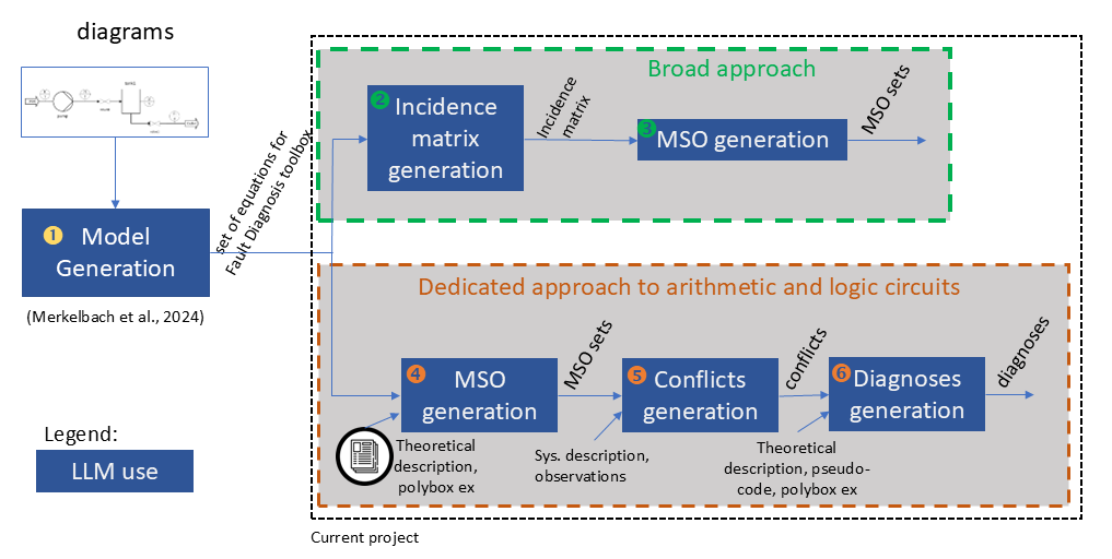
Figure 1 illustrates our methodology. Input to the methodology are P&ID diagrams and circuit diagrams, i.e. a common form of engineering documentation for use-cases in the process industry and hardware design. Block 1 “Model Generation” has been described in [12]. It generates a set of equations that can be used by the Fault Diagnosis Toolbox to obtain MSO sets. Section 4 briefly recalls the model generation process.
For our solution in this article, we used two independent prompting approaches:
-
1.
A Broad Approach (in green box), able to handle continuous systems described by the differential equations that generates MSO sets from a set of differential equations
-
2.
A Dedicated Approach to arithmetic and logic circuits (in orange box) that generates MSO sets, conflicts, and finally obtains diagnoses for the considered system.
Blocks 2 and 3 are used for the Broad Approach, described in Section 5.2. Blocks 4, 5, and 6 are used for the Dedicated Approach to arithmetic and logic circuits, described in Section 5.1. Each block uses an LLM for its reasoning.
In the case of arithmetic and logic circuits, checking the consistency of observations with the model is straightforward and leads to unambiguous answers. In the case of continuous, dynamical systems, in the presence of noise and dynamical fault profiles residual evaluation is more challenging. Therefore, for circuits, we perform all the steps that result in diagnoses (Blocks 4 to 6), and in the Broad Approach we only generate MSO sets (Blocks 2 and 3).
3 Background
A system model typically comprises both unknown variables, denoted by , and known variables , which are measured using sensors.
The variables are partitioned into two categories: differential variables and algebraic variables . Faults affecting the system are explicitly represented by a dedicated vector of parameters . We denote the sets of known variables, unknown variables, and faults by , , and , respectively.
A commonly used representation, known as a semi-explicit Differential Algebraic system of Equations (semi-explicit DAE), for general systems in the continuous-time domain is as follows:
| (1) |
Here, and denote the vectors of unknown variables. The vectors and represent the measured outputs and controlled inputs, respectively, both considered known. In systems without external actuation, may be zero.
The functions , , and can be linear or nonlinear and typically depend on a set of system parameters, denoted by (e.g., tank diameter, nominal flow rate, etc.).
Interestingly, dynamic systems (represented by differential equations) and static systems (represented by algebraic equations) are sub-classes of DAEs.
For any vector , we define as the augmented vector comprising and its time derivatives up to a certain (unspecified) order.
Definition 1 (Analytical Redundancy Relations (ARR)).
ARRs are relations obtained from by formally eliminating unknown variables . While is the internal form that depends on the faults and is not known, is the computation form and can be computed from the known variables and their derivatives.
defines a set of ARRs. A single ARR takes the form , where is a scalar signal named residual and a subvector of . It can be used as residual generator.
Definition 2 (Residual generator for ).
A relation of the form , with input a subvector of and output , a scalar signal named residual, is a residual generator for the model if, for all consistent with , it holds that .
In simple terms, a residual generator produces a signal called a residual, which ideally remains zero when the system operates correctly. Any deviation from zero may indicate the presence of a fault.
From the system model, it is possible to derive Analytical Redundancy Relations (ARRs) by exploiting the inherent analytical redundancy. This is typically achieved through variable elimination techniques, resulting in relations that involve only the known variables. ARRs serve as the foundation for diagnosis tests, enabling the verification of whether the measurements are consistent with the system model . If a fault is present in the system, it is expected to affect some of the measurements, and consequently, the residuals. If no such influence is observable, the fault is said to be non-detectable, and as such, it cannot be identified [9].
Building on the foundational work by Cassar and Staroswiecki [1], and Travé-Massuyès et al. [20], structural analysis has emerged as a powerful tool for deriving ARRs. This method abstracts the system model by focusing solely on the structural relationships between equations and variables, disregarding the specific functional forms. One of the key advantages of structural analysis is its applicability to large-scale systems, whether linear or nonlinear, and even in the presence of model uncertainty. Along the structural approach, the structure of a system , or structural system, can be represented by a biadjacency matrix crossing variables and equations, named the Incidence Matrix.
Definition 3 (Incidence matrix).
The Incidence Matrix of a system is an binary matrix, where is the number of unknown variables, is the number of known variables, and is the number of equations. Each row stands for an equation and each column for a variable. A 1 in position means that the equation of row contains the variable of column .
When applied to fault diagnosis, structural analysis helps identify subsets of equations that exhibit redundancy. The structural redundancy of a set of equations is defined as the difference between the number of equations and the number of unknown variables within that subset.
Of particular diagnostic relevance are the Proper Structurally Overdetermined (PSO) sets, which are sets of equations that together contain just enough redundancy to allow fault detection through consistency checks.
A just determined part refers to a set of equations where the number of equations matches the number of unknown variables, allowing for a unique solution. In contrast, an underdetermined part has fewer equations than unknowns, making it impossible to uniquely determine the values of all variables.
Definition 4 (PSO set).
A subset of equations is a PSO set if its number of equations is greater than the number of unknown variables, and this overdetermination applies to the entire set (i.e., the set is structurally redundant and contains no exactly or underdetermined parts).
Another interesting concept are the minimal subsets of equations that possess exactly one degree of structural redundancy, i.e., . Such subsets are referred to as Minimal Structurally Overdetermined (MSO) sets.
Definition 5 (MSO set).
A subset of equations is an MSO set of if (1) , and (2) no subset of is overdetermined. The set of MSO sets of is denoted .
Certain MSO sets have been shown to support the formulation of diagnostic tests [9], making them essential components for residual generation and fault detection. These particular subsets are called Fault-Driven Minimal Structurally Overdetermined (FMSO) sets [15].
Let denote the set of faults involved in a given subset of equations , then FMSO sets can be defined as follows.
Definition 6 (FMSO set).
A subset of equations is an FMSO set of if (1) is an MSO set and (2) . The set of FMSO sets of is denoted .
Given an FMSO set , is defined as the fault support of and the physical components modeled by the equations in define its component support .
In most cases, FMSO sets can be transformed into Analytical Redundancy Relations (ARRs) through sequential elimination. Due to their structural properties, all unknown variables appearing in an FMSO set can be algebraically resolved using equations. These expressions can then be substituted into the remaining -th equation, yielding an ARR formulated off-line. This ARR is subsequently employed on-line as a diagnostic test.
Building upon the findings in [2], which establish a connection between model-based approaches from the control community (FDI) and those from the artificial intelligence community (DX), the concept of an R-conflict, originally introduced by Reiter [16], can be related to FMSO sets under the assumption of Model Representation Equivalence.
Definition 7 (R-conflict).
The component support of an FMSO set is an R-conflict if the diagnosis test derived from fails when evaluated with the measurements obtained from the physical system. A minimal R-conflict is an R-conflict that does not strictly include (set inclusion) any R-conflict.
An R-conflict indicates that at least one component within the R-conflict must be faulty to explain the observed behavior; equivalently, it is not possible for all components in the R-conflict to be functioning normally. Interestingly, the set of minimal diagnoses can be generated from the set of minimal R-conflicts.
Definition 8 (Minimal diagnosis).
A set of physical components , modeled by some of the equations of , is a minimal diagnosis if and only if it is a minimal hitting 444A hitting set for a collection of sets is a set such that for each . A hitting set is minimal if and only if no proper subset of it is a hitting set for . set of the collection of minimal R-conflicts.
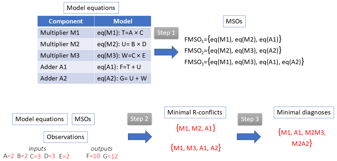
Figure 2 illustrates the different concepts that have been introduced on the well-known polybox example.
The notion of FMSO set also plays a pivotal role in the formal definitions of structural detectable and structural isolable faults. In the following, we revisit these fundamental definitions as presented in [9].
Definition 9 (Detectable fault).
A fault is structurally detectable in the system if there exists an FMSO set such that .
Definition 10 (Isolable faults).
Given two structurally detectable faults and of , , is structurally isolable from if there exists an FMSO set such that and .
The Fault Diagnosis Toolbox (FDT) [5] is a software framework designed for the analysis and synthesis of fault diagnosis in systems that are typically modeled with differential-algebraic equations. By leveraging a structural representation of the system, the toolbox enables the automatic extraction of FMSO sets. From these sets, it allows one to generate Analytical Redundancy Relations (ARRs), which can subsequently be used as diagnosis tests.
4 Model generation
Previous work [12] proposes an approach to create mathematical models for process industry systems using multi-modal large language models (MLLM). It presents a five-step prompting approach that uses a piping and instrumentation diagram (P&ID) and natural language prompts as its input. For clarity, we will briefly sketch the previous approach in this section.
The five steps of the prompting approach are the following:
-
1.
Read Diagram – Let the MLLM read the diagram image data and represent it in some partially specified intermediate format. Partial specification is performed in the prompt.
-
2.
Identify Sensors – The LLM creates a table containing existing sensors, their type, and their placement from the input diagram and from the output from step 1 in the form of . Context about P&IDs, possibly occurring sensors, and the placement of the sensors in the diagram are provided in the system message.
-
3.
Create the mathematical Equations – The mathematical equations are created by the LLM using provided variable names and assumptions.
-
4.
Sensor Matching and Variable Assignment – In this step, all the results from the previous steps are merged, the faults are added to the equations and the resulting mathematical model is created.
-
5.
Format Model for Fault Diagnosis Toolbox – In the final step, the mathematical model is transformed to be suitable for the FDT into .
All steps provide the MLLM with the P&ID as input. In addition, the steps take a system message and a user prompt as input. The system message contains the generic task for the respective step. However, taking current abilities of MLLMs into account, it is still domain dependent. The user message contains a subset of the external information which is specific for the system, where is denotes all available external information. The prompts can be found on GitHub555https://github.com/silkeme/DX24_Model_Creation_LLMs
The repository contains the prompts, all mentioned information about the systems used for the evaluation, the resulting mathematical models, and all intermediate outputs.. The approach aims to work for water tank systems with standard components, such as tanks, pumps, valves, flow indicators, and level indicators.
5 Generating MSO Sets, Conflicts, and Diagnoses
As described before, for our solution in this article, we use two independent prompting approaches:
-
1.
Dedicated approach – designed to handle arithmetic and logic circuits,
-
2.
Broad approach – able to handle continuous systems described by differential equations.
While the Dedicated Approach outputs proper diagnoses, the Broad Approach outputs the more general FMSO sets from which diagnoses can be computed using actual observations and tools such as the Fault Diagnosis Toolbox.
5.1 Dedicated approach to arithmetic and logic circuits
To generate the diagnoses, we test the following approach consisting of three steps:
-
1.
Generation of MSO sets – We provide system equations and the sets of , , and variables as inputs. The model is asked to output all Minimal Structurally Overdetermined (MSO) Sets. This is illustrated by block 4 in Figure 1. Table 1 presents the prompt. The prompt contains a theoretical description and the Polybox system.
-
2.
Generation of Conflicts – We provide the system description, the MSO sets, and observations as inputs. The LLM is asked to evaluate all MSOs for consistency and to generate all conflicts. The prompt contains the theoretical description, detailed steps, and hints for the Python implementation (we test variants with code interpreter allowed) and three simple examples. This is illustrated by block 5 in Figure 1.
-
3.
Generation of Diagnoses – We provide the set of conflicts as inputs. The model is asked to generate all minimal diagnoses. The prompt contains the theoretical description, pseudo-code of the algorithm, and Polybox example. This is illustrated by block 6 in Figure 1.
Figure 3 illustrates the inputs and outputs of each step in the Dedicated Approach (we follow the example from Figure 2). We start with a system description given by a set of equations (system model , Equation 1) and generate MSO sets (Definition 5) using the prompt given in Table 1. Next, residual generators (Definition 2), resulting from each MSO, are evaluated given the values of known variables . The value of a residual generator different from 0 indicates the existence of R-conflict (Definition 7). The output of the second step is the set of conflicts. In the last step, the conflicts are used to generate minimal diagnoses (Footnote˜4).
The prompts for the computation of conflicts and diagnoses can be found on GitHub666https://github.com/asztyber/LLM_diagnostic_concepts/blob/main/prompts/dedicated/prompts_Karol.py The file contains three prompts for the three mentioned steps. Code to run the experiments can be found in https://github.com/jadlownik/FaultDiagnosis/tree/develop.
| Perform an analysis of the equation system equations and identify all Minimal Structurally Overdetermined (MSO) sets. |
| Definitions: |
| 1. Unknown variables: These are only the variables that start with “x”. |
| 2. Structural redundancy: This is the difference between the number of equations and the number of unique unknown variables in those equations: |
| . |
| 3. PSO (Properly Structurally Observable): A subset is PSO if its structural redundancy is greater than . |
| Conditions: |
| 1. The selected set of equations must have exactly one structural redundancy. |
| 2. None of its proper subsets can be PSO (all must have redundancy ). |
| Output: JSON format: { "mso": [...] }, where each inner list represents a valid MSO set. |
| RESPONSE MUST BE IN JSON FORMAT. DO NOT GENERATE CODE AND RETURN IT IN RESPONSE. |
| <example> |
| <input> |
| equations = { |
| ’M1’: ’a * c = x01’, |
| ’M2’: ’b * d = x02’, |
| ’M3’: ’c * e = x03’, |
| ’A2’: ’x01 + x02 = f’, |
| ’A1’: ’x02 + x03 = g’, |
| } |
| </input> |
| <output> |
| { "mso" = [[’M1’, ’M2’, ’A1’], [’M2’, ’M3’, ’A2’], [’M1’, ’M3’, ’A1’, ’A2’]] } |
| </output> |
| </example> |
5.2 Broad approach
To generate the MSO sets, the approach consists of two steps:
- 1.
-
2.
Generation of MSO sets – We provide the incidence matrix including only unknown variables as input. The model is asked to find all the MSO sets for the provided model in two sub-steps. First, find all the PSO sets (Definition 4), then, within these PSO sets, find the minimal ones. Two versions were implemented, one with code interpreter and one without code interpreter. This is illustrated by block 3 in Figure 1. The prompt for the variant without code interpreter is shown in Table 3.

Figure 4 illustrates the inputs and outputs of the two steps for finding the MSO sets. In the first step, the incidence matrix is computed (Definition 3). Only the part containing unknown variables is computed, which is the important part for MSO generation. In the second step, MSOs (Definition 5) are computed from the incidence matrix via PSO sets.
The full set of prompts (including variant for use of code interpreter) can be found on GitHub777https://github.com/asztyber/LLM_diagnostic_concepts/blob/main/prompts/broad/ The directory contains prompts and code to run them..
| Your job is to create an incidence matrix of the provided model. In the incidence matrix, each row represents an equation and each column represents an UNKNOWN variable. Note that unknown variables are stored under key ’x’ in the provided model. |
| Return the incidence matrix. Please return the matrix as a Python dictionary in the following format: ’eq0’: [’unknown var in eq0’, …], ’eq1’: [’unknown var in eq1’, …], … |
| Each line in the dictionary should correspond to one equation (do not write everything on the same line). Only return the dictionary. |
| Be careful with the equations of type ’fdt.DiffConstraint’. Change those equations by a simple equality relation. If you have fdt.DiffConstraint(dt,t), change it by t - dt. Make sure to complete your analysis before responding to me. |
| Your job is to find all the MSO (Minimal Structurally Overdetermined) sets for the provided model, represented here by the provided incidence matrix. In the incidence matrix, each line represents an equation with the unknown variables that belong to this equation. Note that the matrix contains only the unknown variables. MSO sets consist of equations and contain one more equation than the number of unknown variables. |
| Proceed in two parts. First, find all the PSO (Proper Structurally Overdetermined) sets. Then, within these PSO sets, collect those that are minimal (PSO sets that do not contain any subsets that are PSO) to keep only the MSO sets. Store all the MSO sets in a python dictionary and return only the dictionary to me. Use one line for each MSO set. |
| Additionally, include the number of MSO sets found in the dictionary. You MUST only return the dictionary. Don’t make up an example, work with the provided incidence matrix. Make sure to complete your analysis before responding to me. |
6 Test and Validation
All approaches were evaluated through OpenAI API. We evaluated the following models: gpt-4o-mini-2024-07-18 (referred in the following as 4o-mini), o3-mini-2025-01-31 (referred in the following as o3-mini), and o1-2024-12-17 (referred in the following as o1). 4o-mini was evaluated with the access to the code interpreter, therefore the model could write Python code and run it to generate the answer888We tried gpt-4o and gpt-4o-mini but the accuracy was close to zero on unseen examples. Performance of gpt-4o and gpt-4o-mini with code interpreter was similar in initial experiments, so we decided to evaluate full set of examples on gpt-4o-mini because of costs.. o1 and o3-mini are reasoning models999https://openai.com/index/learning-to-reason-with-llms/, trained with reinforcement learning to perform complex reasoning, and performing all computations in internal chain of thought. Note that we cannot tell for sure that these models did not use a code interpreter in the background as well.
Experiments were performed with temperature 0 and top_p = 0 for 4o-mini. The reasoning effort for o1 and o3-mini was ’high’ for the Dedicated Approach and ’medium’ for the Broad Approach. Tests were repeated 10 times for each test case (test case including example description and the set of observations) for 4o-mini and o3-mini. Tests for o1 were performed only once, because of costs101010One iteration costed around 30$.
Each LLM reasoning step was evaluated independently, i.e. for each blue box in Figure 1 we provided correct inputs, irrespective of the result of the previous step. That way, we can evaluate the accuracy of each algorithm step reliably.
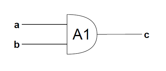
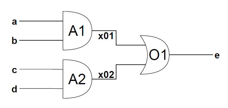
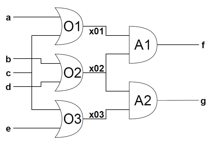
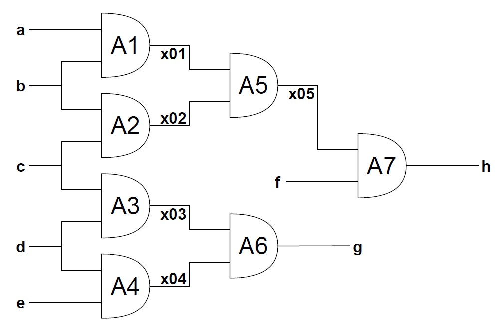
We carried out tests on 23 arithmetic and logic circuits with different levels of complexity (Figure 5). The circuits contain adders, multipliers, and AND, OR, NOR, NAND, and XOR gates. Table 4 summarizes examples’ characteristics111111You can find image for each example here https://github.com/jadlownik/FaultDiagnosis/tree/develop/images and descriptions here https://github.com/asztyber/LLM_diagnostic_concepts/tree/main/examples. The number of minimal conflicts and diagnoses can vary for a given example depending on the observations121212The results contain readable Excel files containing generated and correct MSOs, conflicts and diagnoses.. For each example, we assumed all inputs and outputs are measured. We only considered components faults. Sensor faults and sensor equations were omitted.
| Example | Relations | MSOs | Conflicts | Diagnoses | |||
|---|---|---|---|---|---|---|---|
| Example 2 | 10 | 7 | 5 | 5 | 3 | 0–3 | 0–8 |
| Example 3 | 13 | 8 | 7 | 7 | 2 | 0–2 | 0–12 |
| Example 4 | 13 | 8 | 7 | 7 | 2 | 0–2 | 0–12 |
| Example 5 | 13 | 8 | 7 | 7 | 2 | 0–2 | 0–12 |
| Example 6 | 17 | 11 | 8 | 8 | 3 | 0–3 | 0–21 |
| Example 7 | 13 | 9 | 6 | 6 | 3 | 0–2 | 0–5 |
| Example 8 | 18 | 10 | 11 | 11 | 6 | 0–5 | 0–45 |
| Example 9 | 29 | 17 | 15 | 15 | 6 | 0–6 | 0–165 |
| Example 10 | 3 | 3 | 1 | 1 | 1 | 0–1 | 0–1 |
| Example 11 | 7 | 5 | 3 | 3 | 1 | 0–1 | 0–3 |
| Example 12 | 10 | 7 | 5 | 5 | 3 | 0–2 | 0–5 |
| Example 13 | 13 | 8 | 7 | 7 | 2 | 0–2 | 0–12 |
| Example 14 | 13 | 8 | 7 | 7 | 2 | 0–2 | 0–12 |
| Example 15 | 13 | 8 | 7 | 7 | 2 | 0–2 | 0–12 |
| Example 16 | 17 | 11 | 8 | 8 | 3 | 0–3 | 0–21 |
| Example 17 | 13 | 9 | 6 | 6 | 3 | 0–3 | 0–9 |
| Example 18 | 18 | 10 | 11 | 11 | 6 | 0–5 | 0–57 |
| Example 19 | 29 | 17 | 15 | 15 | 6 | 0–5 | 0–153 |
| Example 20 | 12 | 9 | 5 | 5 | 3 | 0–3 | 0–8 |
| Example 21 | 12 | 9 | 5 | 5 | 3 | 0–3 | 0–8 |
| Example 22 | 7 | 5 | 3 | 3 | 1 | 0–1 | 0–3 |
| Example 23 | 3 | 3 | 1 | 1 | 1 | 0–1 | 0–1 |
| Example 24 | 7 | 5 | 3 | 3 | 1 | 0–1 | 0–3 |
As shown in Figure 6, we evaluate the models’ performance using complementary metrics that capture different aspects of accuracy in incidence matrix generation. For each equation, precision measures how many of the model’s predicted variables are correct, while recall measures how many of the correct variables the model identified. The F1 score combines these into a single metric, penalizing both missing and spurious variables. The accuracy metric is the strictest, requiring perfect variable sets for each equation.
4o-mini often includes known variables and faults as variables involved in incidence matrix, resulting in the poor scores.
Ground truth for incidence matrices, MSO sets, and residual evaluation was computed using Fault Diagnosis Toolbox [5]. Correct minimal diagnoses were computed with the implementation of minimal hitting sets algorithm.
The evaluation metrics (Precision, Recall, and F1 score) were computed by comparing the generated MSO sets with the ground truth MSO sets. Precision measures the fraction of correctly identified MSO sets among all generated sets (), while Recall indicates the fraction of ground truth MSO sets that were successfully found ()131313In the case where the number of ground truth solutions is zero (), and the generated solution is also empty () we set Precision and Recall to 1, to avoid penalizing correct answers for the empty solutions.. The F1 score is the harmonic mean of Precision and Recall (). The metrics for conflicts and diagnoses were computed in an analogous way.
The Figures 8, 10, and 12 show F1 scores for different model versions (4o-mini, o1, and o3-mini). Each data point represents the mean F1 score for examples with the same number of solutions (MSOs, conflicts, or diagnoses), with error bars indicating the standard deviation across these examples. The dashed lines show the linear trend of performance as the number of solutions increases. The Figures 7, 9, and 11 show F1 scores sorted by the number of relations in the example.
7 Discussion
An analysis of the obtained results leads to the following conclusions.
For incidence matrix generation (Figure 6), we can observe that o1 and o3-mini achieve perfect accuracy. 4o-mini tends to include additional variables (not in but correctly assigned to the equations); otherwise, the results are correct. Incidence matrix generation is the simplest algorithmic task.
For MSO generation (Figure 7), 4o-mini has problems with examples containing only one relation. Otherwise, the performance is relatively stable with an increasing number of examples. 4o-mini has access to a code interpreter, making handling different input sizes easier. The performance of o1 and o3-mini decreases with the number of relations in the example. We can observe similar tendencies depending on the number of MSOs to be generated (Figure 8). Plots on Figure 7 and Figure 8 show results aggregated over two prompting approaches (Dedicated and Broad). Figure 13 compares the performance of different models and prompting approaches. The performance of the Dedicated and Broad Approach is similar despite much more domain knowledge included in the dedicated prompts. Additionally, the Broad Approach includes a correct incidence matrix as an input for MSO generation, but it does not influence the results significantly. o1 shows the best performance across all metrics, while 4o-mini is the worst despite the access to the code interpreter.
Performance in conflict generation, depending on the number of relations and conflicts, is presented respectively in Figure 9 and Figure 10. Trend lines show increasing performance with increasing complexity, but this is caused by poor performance when the number of conflicts is zero (i.e. there are no inconsistencies in the system description and observation). o1 performs best for conflict generation (Figure 14).
Diagnoses generation is the most computation-heavy task. We observe a clear decrease in the performance with increasing complexity (Figure 11 and Figure 12). o3-mini performs best for diagnoses generation (Figure 15).
As LLMs were not primarily designed to handle algorithmic and computational tasks, the performance of reasoning models is surprisingly good. o3-mini achieves on conflicts generation and on diagnoses generation. The examples were generated manually and were unavailable in the training data (correct solutions were released after the tested models’ release).
8 Conclusion
This paper explores the use of large language models (LLMs) as a novel tool for performing structural analysis in model-based diagnosis (MBD), specifically focusing on the automatic generation of Minimal Structurally Overdetermined (MSO) sets, from which diagnosis tests can be obtained, from engineering documentation. The generation of conflicts and diagnoses is also explored. The authors evaluate the performance of various OpenAI LLMs (including o1, o3-mini, and 4o-mini) by comparing their generated MSOs, conflicts, and diagnoses against those produced by traditional tools. The paper situates its contribution within a growing body of work on LLM-based fault diagnosis but emphasizes its unique connection to foundational MBD concepts. An empirical evaluation highlights both the potential and limitations of LLMs in structured engineering tasks, offering insights into their applicability and future integration into hybrid diagnostic frameworks.
The main goal of this work is to evaluate LLM capabilities in the context of MBD fault diagnosis. While we find some results surprisingly good, at this point, LLMs do not provide an alternative to diagnosis algorithms. The current level of accuracy is not sufficient to replace traditional tools. Additionally, as the results are obtained by API calls, the time to achieve the results depends on the network load and other factors and cannot be bounded robustly. Another practical consideration is the cost. Lastly, it can be observed that the quality of the results vary highly in different runs.
Several avenues can be explored to extend this work. First, broader benchmarking on more diverse and complex systems, including hybrid systems or distributed systems, would help assess the generalization capabilities and scalability of LLMs in diagnostic tasks. Another promising direction involves fine-tuning or instruction-tuning language models on domain-specific corpora to improve their performance. Additionally, integrating multi-modal inputs – such as P&ID diagrams, circuit schematics, or CAD models – via vision-language models may allow more intuitive and direct processing of engineering data.
Furthermore, future work could explore the use of the recent Model Context Protocol (MCP) in diagnostic frameworks involving distributed architectures. MCP provides a structured way to manage model contexts and execution flows across different computational components. By integrating MCP with language models, it becomes possible to coordinate diagnostic reasoning over a set of specialized servers, each responsible for distinct functionalities – such as structural analysis, variable elimination, or diagnosis generation from conflicts. This would enable a modular and scalable diagnostic pipeline, where LLMs interact with context-aware services rather than operating as monolithic agents. On the other hand, this modular structure is particularly well suited for diagnosis in distributed systems, where different subsystems may operate independently, expose only partial observability, or follow different modeling paradigms. MCP can enable seamless orchestration of context-aware services across these subsystems, allowing LLMs to query relevant components dynamically and integrate partial diagnosis results into a coherent global view. Such an approach enhances scalability, reusability, and flexibility in large-scale or heterogeneous diagnosis environments, while also opening new opportunities for intelligent fault management across distributed infrastructures.
References
- [1] J-Ph Cassar and M Staroswiecki. A structural approach for the design of failure detection and identification systems. IFAC Proceedings Volumes, 30(6):841–846, 1997.
- [2] Marie-Odile Cordier, Philippe Dague, Michel Dumas, François Lévy, Jacky Montmain, Marcel Staroswiecki, and Louise Travé-Massuyes. A comparative analysis of ai and control theory approaches to model-based diagnosis. In ECAI, pages 136–140, 2000.
- [3] Akshay J Dave, Tat Nghia Nguyen, and Richard B Vilim. Integrating llms for explainable fault diagnosis in complex systems. arXiv preprint arXiv:2402.06695, 2024. doi:10.48550/arXiv.2402.06695.
- [4] Teresa Escobet, Anibal Bregon, Belarmino Pulido, and Vicenç Puig. Fault Diagnosis of Dynamic Systems. Springer, 2019.
- [5] Erik Frisk, Mattias Krysander, and Daniel Jung. A toolbox for analysis and design of model based diagnosis systems for large scale models. IFAC-PapersOnLine, 50(1):3287–3293, 2017.
- [6] Sungmin Kang, Gabin An, and Shin Yoo. A quantitative and qualitative evaluation of llm-based explainable fault localization. Proceedings of the ACM on Software Engineering, 1(FSE):1424–1446, 2024. doi:10.1145/3660771.
- [7] Abdullah Khan, Rahul Nahar, Hao Chen, Gonzalo E Flores, and Can Li. Faultexplainer: Leveraging large language models for interpretable fault detection and diagnosis. arXiv preprint arXiv:2412.14492, 2024.
- [8] Mattias Krysander, Jan Åslund, and Mattias Nyberg. An efficient algorithm for finding minimal overconstrained subsystems for model-based diagnosis. IEEE Transactions on Systems, Man, and Cybernetics-Part A: Systems and Humans, 38(1):197–206, 2007. doi:10.1109/TSMCA.2007.909555.
- [9] Mattias Krysander, Jan Åslund, and Mattias Nyberg. An efficient algorithm for finding minimal overconstrained subsystems for model-based diagnosis. IEEE Transactions on Systems, Man, and Cybernetics - Part A: Systems and Humans, 38(1):197–206, 2008. doi:10.1109/TSMCA.2007.909555.
- [10] Karol Kukla. jadlownik/FaultDiagnosis. Software, swhId: swh:1:dir:b8a40cc86347d60c8efb7ce10df9343400eee88e (visited on 2025-10-20). URL: https://github.com/jadlownik/FaultDiagnosis/tree/develop, doi:10.4230/artifacts.24965.
- [11] Lin Lin, Sihao Zhang, Song Fu, and Yikun Liu. Fd-llm: Large language model for fault diagnosis of complex equipment. Advanced Engineering Informatics, 65:103208, 2025. doi:10.1016/J.AEI.2025.103208.
- [12] Silke Merkelbach, Alexander Diedrich, Anna Sztyber-Betley, Louise Travé-Massuyès, Elodie Chanthery, Oliver Niggemann, and Roman Dumitrescu. Using multi-modal llms to create models for fault diagnosis. In The 35th International Conference on Principles of Diagnosis and Resilient Systems (DX’24), volume 125, 2024.
- [13] Herbert Muehlburger and Franz Wotawa. Flex: Fault localization and explanation using open-source large language models in powertrain systems (short paper). In 35th International Conference on Principles of Diagnosis and Resilient Systems (DX 2024), pages 25:1–25:14. Schloss Dagstuhl – Leibniz-Zentrum für Informatik, 2024. doi:10.4230/OASIcs.DX.2024.25.
- [14] Herbert Mühlburger and Franz Wotawa. Faultlines-evaluating the efficacy of open-source large language models for fault detection in cyber-physical systems. In 2024 IEEE International Conference on Artificial Intelligence Testing (AITest), pages 47–54. IEEE, 2024. doi:10.1109/AITEST62860.2024.00014.
- [15] CG Pérez-Zuniga, E Chanthery, L Travé-Massuyès, and J Sotomayor. Fault-driven structural diagnosis approach in a distributed context. IFAC-PapersOnLine, 50(1):14254–14259, 2017.
- [16] Raymond Reiter. A theory of diagnosis from first principles. Artificial intelligence, 32(1):57–95, 1987. doi:10.1016/0004-3702(87)90062-2.
- [17] Alicia Russell-Gilbert, Alexander Sommers, Andrew Thompson, Logan Cummins, Sudip Mittal, Shahram Rahimi, Maria Seale, Joseph Jaboure, Thomas Arnold, and Joshua Church. Aad-llm: Adaptive anomaly detection using large language models. In 2024 IEEE International Conference on Big Data (BigData), pages 4194–4203. IEEE, 2024. doi:10.1109/BIGDATA62323.2024.10825679.
- [18] Anna Sztyber Betley. asztyber/LLM_diagnostic_concepts. Software, swhId: swh:1:dir:d265fcfc25d623bff2fa34d48590c7eb66d08995 (visited on 2025-10-20). URL: https://github.com/asztyber/LLM_diagnostic_concepts, doi:10.4230/artifacts.24966.
- [19] Laifa Tao, Haifei Liu, Guoao Ning, Wenyan Cao, Bohao Huang, and Chen Lu. Llm-based framework for bearing fault diagnosis. Mechanical Systems and Signal Processing, 224:112127, 2025.
- [20] Louise Travé-Massuyes, Teresa Escobet, and Xavier Olive. Diagnosability analysis based on component-supported analytical redundancy relations. IEEE Transactions on Systems, Man, and Cybernetics-Part A: Systems and Humans, 36(6):1146–1160, 2006. doi:10.1109/TSMCA.2006.878984.
- [21] Aidan ZH Yang, Claire Le Goues, Ruben Martins, and Vincent Hellendoorn. Large language models for test-free fault localization. In Proceedings of the 46th IEEE/ACM International Conference on Software Engineering, pages 1–12, 2024.