Using Qualitative Simulation Models for Monitoring and Diagnosis

In 2022, the International Energy Agency estimated the buildings’ energy-related CO₂ emissions at around 27% of the total worldwide CO₂ emissions. To bring the emissions down, several actions have to be taken, including monitoring and diagnosis of heating and cooling systems that often operate in non-optimal operational spaces using far more energy than necessary. This is well visible when considering previous work (i) in the context of radiant ceiling cooling systems, where model predictive control can reduce energy consumption by up to 27% (see, e.g., [10]), or (ii) heat pumps where fault diagnosis can reduce energy loss when detected, diagnosed, and repaired early by about 40% [3]. As a consequence, there is a strong need for automated diagnosis of heating and cooling systems in buildings to reduce the overall CO₂ emissions.

Unfortunately, monitoring and fault localization of such systems is complicated because each building is unique, comprising tailored heating and cooling facilities. When using machine learning, we need either to retrain every model for every building, which is expensive and time-consuming or to find a way to adapt trained models. This similarly holds for physical simulation models that would need to be parametrized for every building. However, the basic principles and their corresponding abstract representation of the behavior of each of the facilities are the same, which follow physical principles. Hence, when being able to represent the behavior of systems that follow physical principles in an abstract way, we can use this for at least detecting faults when monitoring the current behavior of a system.

In this paper, we tackle this challenge and suggest utilizing qualitative reasoning to provide an abstract model of a system that can be used for fault detection and, finally, localization. In particular, we discuss how to use and couple qualitative simulation [20] to ordinary monitoring systems. Rinner and Kuipers [24] already suggested the use of qualitative simulation in monitoring. In contrast, we formally define conformance between the outcome of qualitative simulation and the observations obtained from a system. This formal conformance relationship serves as the basis for detecting faults and may also be of use for fault localization, providing that the qualitative simulation models also capture faulty behavior. The idea is to compare the different qualitative states over time with the abstracted observations. This comparison requires not only abstraction but also specific enhancements. For example, we do not continuously observe the behavior over time but at certain time points. Hence, we might not observe reaching landmarks, which would raise false alarms. Therefore, we need to add reasonable qualitative states to the observations for comparison.

We organize this paper as follows: In Section 2, we discuss related work. Afterward, in Section 3, we introduce a simple tank example, which we use in the rest of our paper for illustration purposes. Section 4 introduces qualitative simulation to be self-contained and discusses conformance in detail. Finally, we conclude the paper.

Qualitative reasoning provides a powerful method for modeling dynamic systems under uncertainty by abstracting continuous variables into symbolic associations. Three formalisms form the foundation [26]: Qualitative Process Theory (QPT) [12], which models physical processes using causality and process activation; Qualitative Physics [15], which uses component-level modeling and constraint propagation to envision possible system behaviors; and Qualitative Simulation (QSIM) [20], which simulates all consistent qualitative trajectories from an initial state using a constraint-based model. QSIM represents system dynamics using Qualitative Differential Equations (QDEs), which abstract sets of Ordinary Differential Equations (ODEs). Starting from an initial qualitative state, QSIM generates a behavior tree by enumerating all possible successor states using a transition table of permissible qualitative changes, and then pruning inconsistent states based on qualitative constraints [21].

QSIM has been extended and applied in various diagnostic frameworks. Subramanian and Mooney [25] extended QSIM to model systems with multiple concurrent faults by associating fault-specific constraints and using constraint-based reasoning to isolate them. Similarly, the $\mathrm{SEXTANT}$ system [23] combines QSIM with the $\mathrm{HS}\text{-}\mathrm{DAG}$ algorithm [14] to compute minimal diagnoses based on behavioral conflicts. Another example is $\mathrm{Mimic}$ [11], a semi-quantitative system that integrates QSIM-style simulation with model-based reasoning for process monitoring. $\mathrm{Mimic}$ identifies faults by detecting discrepancies between simulated and observed behavior, and then tests fault hypotheses by adapting the model. Similarly, $\mathrm{DIAMON}$ [22] combines QSIM with consistency-based diagnosis in a layered monitoring framework. It uses qualitative simulation to detect abnormal behavior and incrementally refines the model abstraction level to isolate the root cause.

Beyond classical QSIM applications, efforts have been made to scale qualitative simulation to more complex hybrid systems. Klenk et al. [16, 17] propose translating a subset of Modelica models into qualitative constraints to enable QSIM-style simulation. The approach reduces spurious trajectories by incorporating continuity, higher-order derivatives, and landmark ordering.

QSIM has been successfully combined with frameworks based on constraints, including Constraint Logic Programming over Finite Domains (CLP(FD)) [2] and Answer Set Programming (ASP) [29]. Wiley et al. [29, 28] demonstrate that robots may autonomously learn qualitative action sequences, such as scaling obstacles or navigating uneven terrain, without requiring accurate quantitative representations of the robot or its environment when using their ASP approach to QSIM called ASP-QSIM.

Our approach builds directly on these QSIM-based diagnosis principles but introduces a conformance-based interpretation of system behavior for system monitoring and fault detection. By exploiting ASP-QSIM, our method identifies deviations between observed system trajectories and simulation-derived qualitative behaviors.

In this section, we illustrate the suggested diagnosis approach considering a tank comprising a pipe where water flows in that has a valve for enabling water flow or stopping it, and a sink for preventing overflowing of the tank. We assume that the sink is designed such that even the amount of water coming from a fully opened input valve can be handled. The overall system has also two sensors. Sensor ${𝐒}_{\mathrm{𝟏}}$ is for indicating that the maximum water level is reached. In this case the valve will be closed. Otherwise, the valve is set to open. Another sensor ${𝐒}_{\mathrm{𝟐}}$ measures whether there is an outflow, which indicates a trouble. The second sensor can be seen as a form of safeguard for the outpipe. Figure 1 graphically depicts the tank example.

A mathematical model of this tank systems comprises one input, i.e., the volumetric flow rate, which fills the tank until reaching the maximum level. If there is still an inflow, then the water will flow through the output of the tank (of course unless it is open and not blocked). The ordinary behavior of this tank example can be modeled as follows: The tank has an area $A$ (e.g., in form of a circle of a given radius $r$ where $A=r^2\cdot \pi$), a maximum height $h_{max}$ where the water should stop, and the height of the tank $h_{top}$, which is higher than $h_{max}$. The inflow $in$ is given in the amount of water per time, i.e., in $m^3/s$. The current volume of water is a function of time $V(t)=h(t)\cdot A$ where $h(t)$ is the current height at time $t$. This volume depends on the sum of the inflows over time, i.e., $V(t)={\int }_0^{t_C}in(t)𝑑t$, and, hence, $\frac{dV(t)}{dt}=in(t)$. If the water reaches the maximum level, the valve should close. If this is not the case the water level reaches the outpipe causing an outflow. This outflow should be the same than the inflow, i.e., $out=in$, and no further water is added to the tank. When implementing this model in a simulation language like Modelica [13], we obtain a behavior like the one depicted in Figure 2. For this behavior we assumed a tank with a radius of 1$m$, a maximum level of 1.2$m$, a top level of 1.5$m$, and a flow rate of 0.001$m^3/s$. Note that we varied the inflow over time using a sinus function. This allows us also to see that the inflow into the tank stops when the valve closes. There are fluctuations of the inflow until reaching the maximum level in Figure 2. Afterward, the inflow is zero without fluctuations.

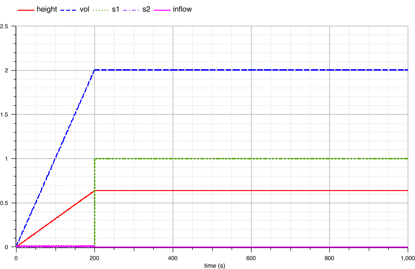
Note that the behavior is similar in case of changed parameters but the steepness of the increase would be different. However, when using concrete values for diagnosis, i.e., the detection and explanation of misbehavior, we need to adapt any comparison function allowing us to show differences between the real and the expected behavior. If we use simulation, we further would need to adapt parameters to fit the simulation outcome with the one of the real systems due to variations between real components and ideal ones. Hence, a qualitative representation of the behavior to be used to check conformance of behavior would be a good idea. To confirm that a water tank system will operate as expected under typical operating conditions, a qualitative simulation using ASP-QSIM was carried out. Figure 3 depicts the qualitative behavior our simulation produces for the tank example. Analyzing the plots, we see that as the tank fills, the inflow progressively decreases and eventually stabilizes at zero, while both volume and water level increase until they reach a maximum state, representing the threshold of the tank. Once this maximum is reached, the sensor ${𝐒}_{\mathrm{𝟏}}$ switched off as expected. Hence, our simulation accurately captures the tank systems nominal behavior.

In the following, we discuss the applicability of qualitative simulation for diagnosis focusing on fault detection. In particular, we want to clarify the following questions:

• $\mathrm{■}$

  What means conformance of a concrete system run and the qualitative simulation result?

• $\mathrm{■}$

  What are the limitations of qualitative simulation when applied for diagnosis? Here, we want to outline limitations considering different fault scenarios. Which type of faults can hardly or not being detected?

For the discussions on limitations, we consider the following fault cases of the tank example, assuming that the fault happens at 200$s$ and remains permanent until the end of simulation:

Fault case 1:

Sensor ${𝐒}_{\mathrm{𝟏}}$ gets stuck at false. In this case, the controller would not get any information and not initiate closing the valve. Hence, the water will reach the outpipe causing sensor ${𝐒}_{\mathrm{𝟐}}$ to go from false to true.

Fault case 2:

Sensor ${𝐒}_{\mathrm{𝟏}}$ is stuck at true, leading to closing the valve immediately. Hence, the tank will not be filled completely.

Fault case 3:

The valve is stuck and always closed leading to zero inflow after 200$s$. Hence, none of the sensor will go to true and the tank cannot be filled.

Fault case 4:

The valve is stuck and remains open. In this case sensor ${𝐒}_{\mathrm{𝟏}}$ indicates reaching the maximum level but having no effect. Hence, the top level is reached and sensor ${𝐒}_{\mathrm{𝟐}}$ will go from false to true.

Fault case 5:

The valve gets stuck at 50% leading to continuous and not stopping inflow. Both sensor indicate reaching a certain water level but the water inflow does not stop.

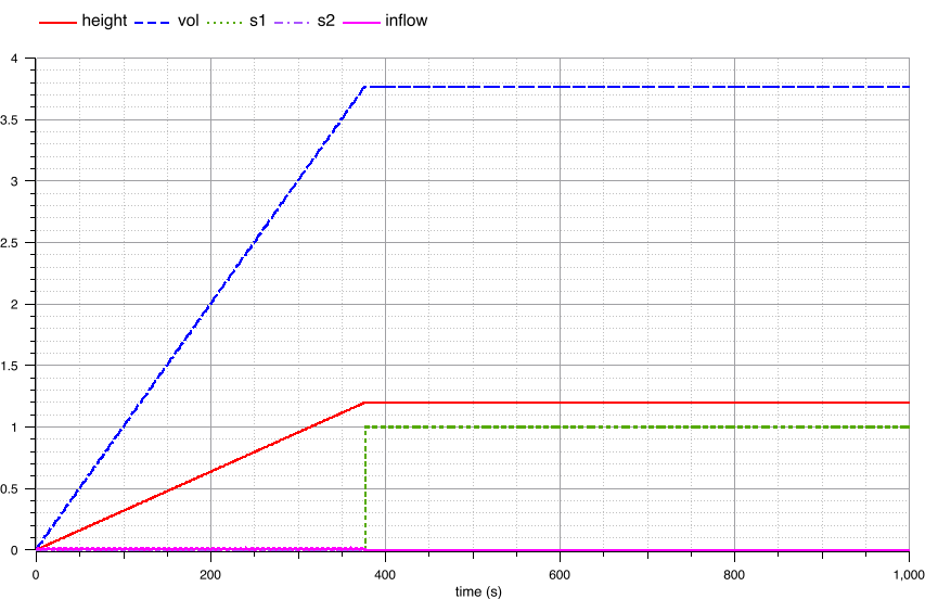
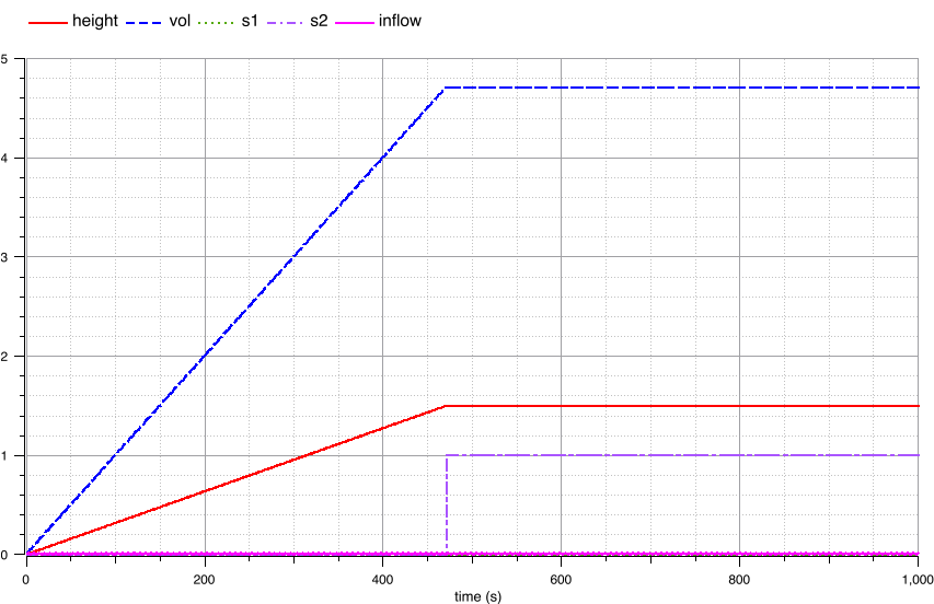
Figure 4 shows the faulty behaviors resulting from the different fault cases. Before discussing the limitations and challenges, we introduce the basic definitions of qualitative simulation in the next section of this paper.

QSIM provides a formal basis for reasoning about physical systems in situations where precise numerical data is unavailable or not needed. Unlike numerical simulation techniques, which require precise parameter values, in QSIM continuous variables are abstracted into symbolic categories such as increasing, decreasing, or landmark values. QSIM simulates all possible behaviors of a system given a qualitative model. Its inputs are: (1) QDEs represented by variables and constraints, and (2) an initial state. QSIM completes the initial state by solving a constraint satisfaction problem (CSP) over the QDEs. For each consistent state, it then generates all valid successors and filters them using constraint consistency. Rather than predicting a single numeric outcome or trace of a simulation, QSIM captures all plausible system behaviors over time [20].

Each variable in a qualitative model is described over a symbolic structure called a quantity space. This space consists of key reference points in the domain of the variable, denoted as landmarks, and the intervals between them. Landmarks represent semantically meaningful thresholds without requiring precise numeric values. We formalize the quantity space as follows.

Based on the quantity space of a variable, we can now define its qualitative value at a particular time step $t$:

These qualitative values form the building blocks of a system’s qualitative state, which captures the complete system snapshot at a given time:

The collection of the qualitative values of all the variables in a system at a given point in time is its qualitative state [30].

By abstracting quantitative system behavior into qualitative representations, we demonstrated how qualitative simulation can effectively detect anomalies across various scenarios by formally defining conformance between the qualitative simulation and concrete quantitative data. At the same time, our evaluation uncovered important limitations. In particular, the exclusion of directional information hindered the detection of one of the faults, which might have been caught had directionality been preserved during abstraction. This highlights a central problem of exclusively qualitative models, even though they can capture high-level patterns and behavior, they may not be able to detect defects that depend on small or deliberate aberrations.

However, the power of qualitative simulation is in its ability to provide a methodical and understandable approach to diagnosis, especially in situations where complete quantitative data is unavailable or unreliable. When considering fault scenarios, it offers a model-based foundation and excels at identifying anomalies and discrepancies across different system behaviors.

Future improvements could include the integration of directional cues to enhance sensitivity to small or gradual deviations, which are currently lost in the reduced abstraction. While the exclusion of the direction of changes simplifies the qualitative behavior space and reduces computational overhead, selectively reintroducing it either for specific variables or during suspected fault windows could strike a balance between fidelity and tractability.

Additionally, the development of hybrid approaches that combine qualitative and quantitative reasoning [4] could further improve fault detection robustness. Such methods may allow the system to benefit from the interpretability and flexibility of qualitative models, while leveraging quantitative models for precision in ambiguous or borderline cases.

Another area of enhancement lies in the application of bounded conformance not just as a binary check but as a tool for localizing faults temporally within the trace. By identifying the prefix length at which divergence from expected behavior occurs, diagnosers could potentially infer the onset time and probable subsystem associated with the deviation. To address the challenge of “silent” faults failures that do not result in a change of qualitative state and thus evade detection future work could explore the use of context-aware thresholds, state persistence checks, or anomaly scoring models that monitor for suspicious invariance in critical variables.

Moreover, QSIM may generate spurious or physically implausible trajectories, particularly in more complex systems. Incorporating domain knowledge, constraint filtering, or ranking heuristics will therefore be crucial for scaling the approach to real-world applications.

References

- [1] Bernhard K. Aichernig, Harald Brandl, and Franz Wotawa. Conformance testing of hybrid systems with qualitative reasoning models. Electronic Notes in Theoretical Computer Science, 253(2):53–69, 2009. Proceedings of Fifth Workshop on Model Based Testing (MBT 2009). doi:10.1016/j.entcs.2009.09.051.
- [2] Aleksander Bandelj, Ivan Bratko, and Dorian Suc. Qualitative simulation with clp. In Proceedings of the 16th International Workshop on Qualitative Reasoning (QR02), 2002.
- [3] I. Bellanco, E. Fuentes, M. VallÚs, and J. Salom. A review of the fault behavior of heat pumps and measurements, detection and diagnosis methods including virtual sensors. Journal of Building Engineering, 39:102254, 2021. doi:10.1016/j.jobe.2021.102254.
- [4] Daniel Berleant and Benjamin J. Kuipers. Qualitative and quantitative simulation: bridging the gap. Artificial Intelligence, 95(2):215–255, 1997. doi:10.1016/S0004-3702(97)00050-7.
- [5] Armin Biere, Alessandro Cimatti, Edmund M. Clarke, Ofer Strichman, and Yunshan Zhu. Bounded model checking. Adv. Comput., 58:117–148, 2003. doi:10.1016/S0065-2458(03)58003-2.
- [6] Harald Brandl, Gordon Fraser, and Franz Wotawa. Qr-model based testing. In Proceedings of the 3rd international workshop on Automation of software test, pages 20–17, 2008.
- [7] Harald Brandl, Martin Weiglhofer, and Bernhard K. Aichernig. Automated conformance verification of hybrid systems. In Ji Wang, W. K. Chan, and Fei-Ching Kuo, editors, Proceedings of the 10th International Conference on Quality Software, QSIC 2010, Zhangjiajie, China, 14-15 July 2010, pages 3–12. IEEE Computer Society, 2010. doi:10.1109/QSIC.2010.53.
- [8] Ivan Bratko. Learning Qualitative Models. Pearson Education, 4 edition, 2012.
- [9] Bert Bredeweg, Floris Linnebank, Anders Bouwer, and Jochem Liem. Garp3 — workbench for qualitative modelling and simulation. Ecological Informatics, 4(5):263–281, 2009. Special Issue: Qualitative models of ecological systems. doi:10.1016/j.ecoinf.2009.09.009.
- [10] Qiong Chen and Nan Li. Model predictive control for energy-efficient optimization of radiant ceiling cooling systems. Building and Environment, 205:108272, 2021.
- [11] Daniel Dvorak and Benjamin Kuipers. Process monitoring and diagnosis: a model-based approach. IEEE expert, 6(3):67–74, 1991. doi:10.1109/64.87688.
- [12] Kenneth D. Forbus. Qualitative process theory. Artificial Intelligence, 24(1-3):85–168, December 1984. doi:10.1016/0004-3702(84)90038-9.
- [13] Peter Fritzson. Modelica - a language for equation-based physical modeling and high performance simulation. In Proceedings of the 4th International Workshop on Applied Parallel Computing, Large Scale Scientific and Industrial Problems, PARA ’98, pages 149–160, London, UK, UK, 1998. Springer-Verlag. doi:10.1007/BFB0095332.
- [14] Russell Greiner, Barbara A. Smith, and Ralph W. Wilkerson. A correction to the algorithm in Reiter’s theory of diagnosis. AI, 41(1):79–88, 1989. doi:10.1016/0004-3702(89)90079-9.
- [15] Johan De Kleer and John Seely Brown. A qualitative physics based on confluences. Artificial Intelligence, 24(1-3):7–83, December 1984. doi:10.1016/0004-3702(84)90037-7.
- [16] Matthew Klenk, Johan de Kleer, Daniel G. Bobrow, and Bill Janssen. Using modelica models for qualitative reasoning. In Proceedings of the 27th International Workshop on Qualitative Reasoning (QR 2013), pages 1–8, 2013.
- [17] Matthew Klenk, Johan de Kleer, Daniel G. Bobrow, and Bill Janssen. Qualitative reasoning with modelica models. In Proceedings of the Twenty-Eighth AAAI Conference on Artificial Intelligence, pages 1084–1090. AAAI Press, 2014. doi:10.1609/AAAI.V28I1.8876.
- [18] Benjamin Kuipers. The limits of qualitative simulation. In IJCAI, 1985.
- [19] Benjamin Kuipers. Qualitative reasoning: Modeling and simulation with incomplete knowledge. Automatica, 25(4):571–585, July 1989. doi:10.1016/0005-1098(89)90099-X.
- [20] Benjamin J. Kuipers. Qualitative simulation. Artificial Intelligence, 29(3):289–338, 1986. doi:10.1016/0004-3702(86)90073-1.
- [21] Benjamin J. Kuipers. Qualitative simulation, 2001. In Encyclopedia of Physical Science and Technology, pages. 287–300.
- [22] Franz Lackinger and Wolfgang Nejdl. Integrating model-based monitoring and diagnosis of complex dynamic systems. In John Mylopoulos and Raymond Reiter, editors, Proceedings of the 12th International Joint Conference on Artificial Intelligence. Sydney, Australia, August 24-30, 1991, pages 1123–1128. Morgan Kaufmann, 1991. URL: http://ijcai.org/Proceedings/91-2/Papers/074.pdf.
- [23] Bruno Lucas, Jean Michel Evrard, and Jean Pierre Lorre. A qualitative diagnosis method for a continuous process monitor system. In Proceedings of the IMACS International Workshop on Qualitative Reasoning and Decision Technologies -QUARDET’93. CIMNE, 1993.
- [24] Bernhard Rinner and Benjamin Kuipers. Monitoring piecewise continuous behaviors by refining semi-quantative trackers. In Thomas Dean, editor, Proceedings of the Sixteenth International Joint Conference on Artificial Intelligence, IJCAI 99, Stockholm, Sweden, July 31 - August 6, 1999. 2 Volumes, 1450 pages, pages 1080–1086. Morgan Kaufmann, 1999. URL: http://ijcai.org/Proceedings/99-2/Papers/059.pdf.
- [25] Siddharth Subhramanian and Raymond J. Mooney. Multiple fault-diagnosis using general qualitative models with fault modes. In Working Papers of the 5th International Workshop on Principles of Diagnosis, pages 321–325, New Paltz, NY, October 1994.
- [26] Louise Travé-Massuyès, Liliana Ironi, and Philippe Dague. Mathematical foundations of qualitative reasoning. AI Magazine, 24(4):91–106, 2003. doi:10.1609/AIMAG.V24I4.1733.
- [27] Jan Tretmans. Conformance testing with labelled transition systems: Implementation relations and test generation. Comput. Networks ISDN Syst., 29(1):49–79, 1996. doi:10.1016/S0169-7552(96)00017-7.
- [28] Timothy Wiley, Claude Sammut, and Ivan Bratko. Using planning with qualitative simulation for multistrategy learning of robotic behaviors. In Proceedings of the 27th International Workshop on Qualitative Reasoning, pages 24–30, 2013.
- [29] Timothy Wiley, Claude Sammut, and Ivan Bratko. Qualitative simulation with answer set programming. In European Conference on Artificial Intelligence (ECAI), May 2014.
- [30] Timothy Colin Wiley. A planning and learning hierarchy for the online acquisition of robot behaviors, 2017. PhD Thesis Defence Paper.