Towards Predictive Maintenance in an Aluminum Die-Casting Process Using Deep Learning Clustering and Dimensionality Reduction
 Luis Ignacio Jiménez
Daniel López
Belarmino Pulido111Corresponding author
Carlos Alonso-González
Luis Ignacio Jiménez
Daniel López
Belarmino Pulido111Corresponding author
Carlos Alonso-González
Abstract
In the manufacturing industry, predictive maintenance requires the estimation of the health status of key subsystems or components. In this study, we will look for degradation patterns in the piston of an injection machine used in an aluminum die casting process operating in an automobile factory in Valladolid (Spain). The injection machine produces a new engine block every 90 seconds and each injection device provides 2000 measurements of various physical variables. This study faced the challenge of finding piston head degradation patterns for an injection machine in the factory, using time series data obtained from the controller, as a preliminary step to estimate the remaining useful life (RUL) of the piston head. The proposed solution used advanced deep learning clustering techniques to generate an index related with the progression of the degradation of the components. The results indicated that degradation patterns can be identified. Later on, using an exponential function an approximation of the RUL can be provided to the plant operator to achieve an ordered piston replacement.
Keywords and phrases:
Prognostics, Deep Learning, Clustering, UMAP, LOWESS regressionFunding:
Miguel Cubero: M. Cubero’s work has been supported by the 2024 Investigo Programme from the Spanish Ministerio de Trabajo y Economia social using EU Next Generation Funds.Copyright and License:
2012 ACM Subject Classification:
Computing methodologies Cluster analysis ; Computing methodologies Dimensionality reduction and manifold learningAcknowledgements:
Authors want to thank our former students David Garcia de Vicuña López de Ciordia and Daniel Veganzones for their help in early stages of this work; also, authors want to acknowledge the people from the Informatics and Injection Sections of the factory for granting access to the time series dataset, and for the help and support provided in understanding the injection process.Funding:
This work has been partially supported by Spanish Ministerio de Ciencia e Innovación under Grant PID2021-126659OB-I00.Editors:
Marcos Quinones-Grueiro, Gautam Biswas, and Ingo PillSeries and Publisher:
1 Introduction
Predictive manufacturing is one of the basic pillars of smart factories under the Industry 4.0 paradigm. This task is essential to improve industry competitiveness [23] and intelligent systems are required to obtain “self-awareness”, “self-predicting”, “self-maintaining”, and “self-learning”, which are inherent capabilities of predictive manufacturing [16]. Health Management Systems (HMS) provide the conceptual framework to build these intelligent systems, which must include all the necessary (and cooperating) tasks to get those capabilities: health state estimation, monitoring, fault detection and diagnosis, prognostics, and predictive maintenance. Prognostics and Health Management (PHM) is the technology commonly used to develop HMS. Such technology aims to detect incipient faults, perform fault diagnosis, and prognostics of failure [3]. Different authors have identified different tasks as essential to develop PHM solutions [3, 1], being the most common: Human-Machine Interfaces, data acquisition, detection, diagnostics, and prognosis modules. In this work we will focus mainly on fault prognostics and predictive maintenance, aiming to extend the useful life of the system, and helping in the optimization of maintenance activities [20].
There are two main approaches to solve the PHM problem: model-based and data-driven [4, 24]. Model-based prognostics [8] use physics-based models that model physical phenomena in order to predict how failure in a system or in its components will evolve. The task has two steps: damage estimation, and damage prediction, which projects the current health state forward in time to determine the End of Life (EOL), and the Remaining Useful Life (RUL) of the system or component. Meanwhile, data-driven prognostics use available data to build a black-box model for predicting the fault growth [10, 25]. In order to extract features from the data that can be related to fault growth [19] different techniques can be used, such as regression (e.g., Gaussian process regression), mapping (e.g., neural networks), or statistics (e.g., relevance vector machines).
In the context of automotive industry, several subsystems or some of their components are so complex that it is not possible to obtain accurate or usable first-principles models. However, in smart factories, with their Cyber-Physical systems (CPSs), large amounts of data are available, specially from a large variety of sensors or automata. The big data obtained from those CPSs can be used to produce data-driven models for HMS purposes; but such kind of models for large parts of a factory are hardly feasible. Instead, using a divide and conquer strategy, smaller models for specific parts of the process or for specific high-level tasks in the HMS (such as fault diagnosis or prognostics) can be obtained. In discrete manufacturing, this is not a major problem because different stages can be clearly isolated.
More specifically, in the domain of automotive manufacturing, several stages can be clearly identified: the production of components (such as engines, gearboxes, etc.), wielding, painting, and assembly. In addition, we can also identify several discrete processes within each stage. This study focuses on one of these processes, required for producing car engines: the aluminum die-casting process, which produces engine blocks. This process is so complex that it is divided into different phases, one of them being the injection of aluminum to produce each engine block. A new aluminum engine block is produced in less than two minutes using an injection machine, whose components also suffer from wear, especially moving parts such as pistons, which are subjected to extreme temperature and pressure conditions. The automatic controller, embedded in each injection machine, measures several physical variables during each aluminum injection. These process measurements for each engine block are stored in the real time database as time series, together with some static data related to the whole injection process, which are stored for maintenance purposes.
In this context, the research questions in this work were: first, is it possible to find degradation patterns for pistons involved in the aluminum die-cast injection process, using only the time series related to physical variables provided by the controller? Second, can we perform an estimation of the RUL for the piston in the injection machine? To answer the first question the calculation of a Fuzzy Progression Index (FPI) is proposed; this index shows the evolution of the piston head wear in sequential stages, combining Autoencoders, dimensionality reduction, and fuzzy clustering. The answer to the second question, the FPI values were used to estimate the current wear state of the piston head, and a projection of its remaining life span.
This study has been done using real data from an automotive factory in Valladolid, Spain; more specifically from one of its injection stations during a three months period in 2023 where abnormal degradation patterns were suspected. From a factory management point of view, finding those degradation patterns would help the predictive maintenance of the system, thus reducing the downtime of the process due to pistons failures.
This manuscript is organized as follows: next section will provide a description of the real case study used in this work. Later, background on the main techniques used in this work will be introduced. Section 4 is focused on the proposal for the estimation of the wear condition of the piston heads, while Section 5 will explain how to obtain an estimation of the RUL for each piston head. In both sections we will provide the results on the case study. Finally, some conclusions will be drawn.
2 Case study: the aluminum die-casting process in an automotive factory in Valladolid, Spain
2.1 The injection process
Car manufacturing has several stages: Stamping (which creates the vehicle basic outer shell out of large rolls of sheet metal), Body Shop (which is devoted to welding and the assembly of the stamped panels from the previous stage), Painting of the car body, Assembly Line (where wiring, electronics, windows, seats, etc. are assembled), Powertrain Assembly (where engines and transmissions are installed), Quality Control and Testing, and finally Logistics and Delivery. In addition, all the components required in these stages need to be produced, such as engine blocks or gearboxes, before they can be assembled. Usually there are whole factories devoted to the production of an specific element, such as the engine block.
This work is focused on the die-casting process, where injection machines produce engine blocks from aluminum ingots, as can be seen in Figure 1. This work aims to build an intelligent system to support quality control for the die-casting process, by means of a degradation model, which can be used to warn the plant operator when the RUL of the system is close. After the die-casting process, the produced engine blocks are tested in the factory before they are delivered to the Powertrain Assembly stage.

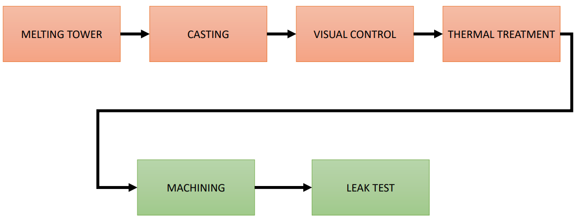
Aluminum die-casting has several stages itself, which can be seen in Figure 2: the aluminum is melted in a Melting tower, and it goes directly to the Casting stage; afterwards, the engine blocks pass a Visual inspection; later on, each engine receives a Thermal treatment to avoid leakages, and the exceeding aluminum is removed in the Machining stage. Finally, to find potential liquid or gas leakages, each engine passes through the Leakage test. Engine blocks that do not pass this test are sent backwards to the Melting tower.
Filling the mold is a process which also has several stages: first, the aluminum is fed into the piston chamber. Second, there is a slow-speed phase, where the piston moves slowly to almost completely fill the mold. Third, there is the low pressure, high-speed phase to completely fill the mold. Fourth, compaction stage uses high pressure to remove air or any other gas from the mold. Later on, a vaccum valve is used to seal the mold. During all these phases, the piston speed and pressure must be carefully controlled, because it is critical to produce fine engine blocks. Finally, once the mold is open again, a layer of an oil-based solution is sprayed on both the engine block, and the mold. Then, there is a cooling stage.
In this study, the information used belongs to three of the four initial stages: slow-speed, high-speed, and compaction. All the data used from these stages are provided by the injection machine.
2.2 The dataset
Each injection lasts less than 90 seconds, and in that span each injection device produces 2000 data for at least five measured signals for each piston: the space traveled, the current speed and its desired set point, and finally, the pressure exerted by the piston on the mold and its desired set point. Consequently, for each injection process, we have five time series made up of 2000 points each222Details about measurement units and scales are intentionally omitted due to confidentiality issues.. In addition, the injection machine provides a text file summarizing the injection process, and accordingly it labels each new engine block. If the generated label is not OK, then the engine block is rejected, but most of the generated engines are labeled as OK.
Figure 3(a) shows the evolution of the five measurements recorded for the relevant parts of one injection: the end of the slow speed, together with the fast speed, and the compaction stages, as described in Section 2.1. However, depending on the settings fixed by each plant operator, the time series had different parameters regarding the initial time point to be measured, and the sampling time for the data series. Hence, we were forced to subsample the original 2000 points to have the same number of points, with reference to the same time instant, for all the injections. Consequently, the time series were reduced to 158 points comprising the end of the slow-speed and the whole fast-speed stages for all the engine blocks. After analyzing those data, the size of the time series was later reduced to 56 points, available from the beginning of the fast-speed stage in the injection. Figure 3(b) shows the 56 points for the same injection as in Figure 3(a).
After training several Deep Learning configurations [7] only 20 time steps were considered as relevant to distinguish different behaviours. From these reduced data, only the real speed () and the real pressure (), measurements were considered relevant. Additional features, related to the temporal evolution of these two measurements were included. Each feature will provide an additional 20 points time series for both and .
-
the standard deviation (five points sliding window), ,
-
relative speed: , ,
-
curvature: , ,
-
third order difference: , ,
-
and lags of order 1 to 5: , .
As a result, the dataset is made up of 20 time series, made up of 20 time steps each, for each engine block: .


The dataset comprised data about engine blocks produced over a three-months span (mid-January to mid-April, 2023) by a single injection machine, and labeled as OK by the device. 20 pistons were used during that period of time, but the factory reported that four of them did not meet the expected lifespan standard, and were replaced due to unforeseen issues (the remaining 16 exhibited normal lifespans). A filtered dataset was established based on these 16 pistons, resulting in a total of 29158 engine blocks. The generated dataset has dimensions , with representing the 29158 engine blocks, indicating the time points collected for each time series, 20, and representing the number of time series used for each block, 20.
3 Background: unsupervised machine and deep learning methods
Raw data is made up of five time series for each engine block, without labels on the different stages of the life cycle of the piston to perform classified supervision, or numerical information on the RUL of each engine block to train a regressor. Hence, it was necessary to look for clusters on the time series previously described (the filtered speed and pressure, plus the nine additional features, such as relative speed, curvature, etc., for each one of them).
Traditional time series clustering techniques can be used to find clusters for different behaviors, partitioning the original data series using different distance or dissimilarity measurements among the series, or features extracted from them. A detailed review of classical techniques for time series clustering can be found in the work by Maharaj et al. [14].
Several classic methods were tested on the current dataset with no satisfactory results [9], being unable to find significant difference between nominal and faulty behavior. Moreover, using supervised deep-learning and information about the early and final stages of the piston life cycle it was possible to separate both stages with more than of accuracy [17], but it was not possible to isolate other degradation stages with more than of accuracy. Consequently, different surveys on deep learning clustering techniques were explored [22, 2, 13, 12], where different methods are proposed; the most common being the combination of autoencoder followed by clustering of the latent space, and transformer-based embeddings also followed by clustering. In the remainder of this section the methods and techniques selected for this work will be summarized. It was decided to use the most promising one for time-series clustering following [12].
3.1 Autoencoder
An autoencoder is a deep neural network designed to learn an efficient representation of the input data, , by means of an Encoder, , that extracts the inputs features to a latent representation, , and then uses a Decoder, , which reconstructs from the encoding , while minimizing a loss function , which measures the difference between the input () and the reconstructed output (). This can be expressed as follows:
| (1) | |||||
| (2) | |||||
| (3) |
The behavior of the autoencoder can be summarized as:
| (4) |
where and are activation functions, are weight matrices and are the biases.
A Dilated Convolutional Neural Network (DCNN) architecture [11] is employed to implement the autoencoder model for time-series clustering. This architecture leverages variations in the dilation parameter, which are determined by the length of the input time series. Specifically, the dilation increases exponentially: at a rate of 4 for series shorter than 50 data points, and at a rate of 2 for longer series.
3.2 Dimensionality reduction
Uniform Manifold Approximation and Projection (UMAP) [15] is a non-linear stochastic method based on graphs for dimensionality reduction. The algorithm is divided into two main steps. First, it constructs a fuzzy graph between the data points: it computes a k-nearest neighbor graph and then defines the probability that two points are connected. Next, it creates the low-dimensional embedding by minimizing a cross-entropy loss, which pulls points together or pushes them apart depending on their distances in the high-dimensional space. This optimization is performed using stochastic gradient descent.
Let be the set of all connections in the graph constructed from the high-dimensional space. Let and denote the weights of a connection in the high- and low-dimensional spaces, respectively. The cross-entropy is then computed as:
| (5) |
The objective is to minimize this function. The first term is minimized by increasing , meaning the points are close together in the low-dimensional space. The second term is minimized by decreasing , which pushes the corresponding points farther apart.
One major advantage of UMAP over other dimensionality reduction methods, such as t-SNE [21], is that, by saving the model parameters, we can obtain the latent representation in the low dimension space for each new block, without recomputing the UMAP model on the whole training set.
UMAP includes several hyperparameters, such as the number of neighbors, the distance metric used to construct the graph, the minimum allowed distance among points in the embedding, and the target dimensionality.
In this work, UMAP will be applied to the latent space from the autoencoder, to reduce its initial dimensionality, which is 50.
3.3 Clustering method
Fuzzy c-means (FCM) [18, 5] is a clustering technique that allows the probabilistic assignment of an element to a set of clusters based on a minimization function. While there are several proposals for optimization criteria, the most popular to date is associated with the least square error function (6).
| (6) |
Where is the number of samples; is the number of clusters, is the degree to which element belongs to the cluster , is the fuzzy factor, strictly greater than one, and is understood as the euclidean distance that separates the element from the centroid of the cluster . Optimization is subject to the constraint and solved using Lagrange multipliers. It is worth mentioning that if tends to one, the optimal partition is increasingly closer to an exclusive partition (K-means), and when it tends to infinity the optimal partition approaches a matrix with all its values are equal to . Usually takes values in the range between .
In this work fuzzy c-means will be applied to the reduced space obtained after applying UMAP to the autoencoder latent space.
3.4 LOWESS
In order to plot the evolution of the cluster assignment obtained after applying fuzzy c-means for each new engine, which will be a really noisy value, LOWESS was selected to smooth the visualization.
LOWESS, which stands for Locally Weighted Scatterplot Smoothing [6], is a robust locally weighted regression method for smoothing scatterplots. Local regression is a nonparametric approach for estimating a regression function or a surface.
Let’s say that we have a collection of points , in a two dimensional space, in which the fitted value at is the value of a polynomial fit to the data using weighted least squares, where the weight for (, ) is larger if is closer to and is smaller if it is not. This fitting procedure is used to deal with deviant points distorting the smoothed points.
In this work LOWESS was applied to the projection on a two, or three, dimensional space for the UMAP output after applying fuzzy c-means.
4 Estimating the wear condition of the piston head with a Fuzzy Progression Index and results on the case study
This section presents a methodology capable of estimating the degree of wear of a piston head throughout its life cycle. For this purpose, a fuzzy index, Fuzzy Progression Index, FPI, was proposed. FPI represents the wear state of the piston head. Information on the piston wear state is not available in the training data, and there are only data related to the number of injections performed by the piston in its life cycle. For these reasons, advanced clustering techniques were chosen to obtain the FPI of a piston throughout its life cycle. This section is devoted to presenting the proposed methodology from the raw data, indicating the processing steps, and showing the experimental results obtained on the training set. The next section will present the methodology to estimate the RUL of a piston from its FPI.
4.1 Experimental setup
The methodology for obtaining the FPI that shows the evolution of piston head wear consists of three sequential stages, which are represented in Figure 4.
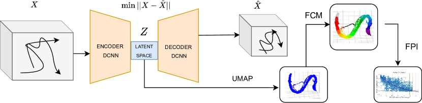
In the first stage, a DCNN-based autoencoder architecture is used to construct a latent representation of the input data. The autoencoder, using dilated convolutions, is trained to minimize the reconstruction error, thereby ensuring that the latent space effectively captures the most relevant features of the original high-dimensional dataset, including local and contextual patterns that might otherwise be lost with standard convolutional layers.
In the second stage, the dimensionality of the latent space generated by the autoencoder is further reduced using Uniform Manifold Approximation and Projection, which provides a compact and computationally tractable representation of the data while preserving its underlying topological structure. In this study, the UMAP projection will generate a three-dimensional region of high point density. The projection of the head piston for each newly generated engine block shifts from one end of the region to the other, as the number of injected blocks increases. Unfortunately, the displacement within the region is noisy, and there is no simple correlation between the location of the projection in one region and the degree of wear.
Finally, in the third stage, due to the noisy evolution of the piston head projection, fuzzy clustering is performed on the reduced latent space using the FCM algorithm. This step groups the engine blocks into distinct overlapping clusters. The trend of assignment of each component to different clusters, based on the probabilities provided by the FCM, can be used to define the Fuzzy Progression Index as follows:
| (7) |
Where is the number of clusters, is the cluster associated with the initial state, is the cluster representing the final state, and is the degree of membership to cluster .
FPI is correlated to the remaining percentage of life of the piston head, but unfortunately it also presents a high variance. Therefore, LOWESS [6] method will be used to smooth the data in order to obtain the trend of the FPI. The resulting curve serves as an indicator of the piston life trend. Using the probabilistic nature of FCM assignments, the approach captures the gradual transition between health states.
Table 1 summarizes the parameter configurations explored for the DCNN, UMAP, and FCM techniques. For the FCM method, the values listed represent the various configurations tested during the optimization process, which aims to improve the accuracy and stability of the cluster assignments across the component data. By systematically adjusting these parameters, the model seeks to enhance the clarity of the clustering structure, ensuring that the transitions between health states are captured more effectively. This cluster representation can be used to obtain a more robust representation of the component’s behavior over time, providing a reliable foundation for subsequent analyses and decision-making processes. This idea will be explained in Section 5.
| Autoencoder | |
|---|---|
| Input sequence length | 20 |
| Latent space dimension | 50 |
| Reconstruction loss functions | MSE |
| DCNN parameters | |
| Dilation | 1, 4, 16 |
| Kernel size | 3 |
| Number of filters | 40 |
| Number of conv. layers per dilation value | 2 |
| Number of filters in the last convolution | 320 |
| UMAP | |
| Number of output dimensions | 3 |
| FCM | |
| Number of clusters | 5–25 |
| Fraction of the data used when estimating each value | 0.3, 0.5, 0.7, 0.9 |
| Fuzzy factor | 2, 2.5 |
4.2 Results for the FPI computation and cluster assignment on the case study
To validate the proposed approach, the dataset was partitioned into training and test subsets, following an 80-20% split, to ensure a fair comparison. The reader should notice that the split was made at the piston level, i.e. we used for training all the measurements from 80% of the available pistons, and 20% of the pistons were used for test, rather than doing a random 80-20% split of available measurements for each piston from the full set of pistons data. As a result, a piston split forms the basis for this work.
Several model configurations were explored for the training set. The upper part of Figure 5(a) shows the resulting structure of the latent space generated by the autoencoder in three dimensions for the training set; this structure can be interpreted as the characteristic life cycle of a piston.


Once the structure was fixed, various numbers of clusters were explored, ranging from five to twenty-five. This range was selected based on preliminary analyses, which indicated that fewer than five clusters failed to capture the necessary complexity of the system degradation patterns, while more than twenty-five clusters led to over-fitting and decreased generalization performance. From these experiments, the optimal number of clusters was determined to be 23, as this configuration achieved the best performance in the FCM method of FPI optimization. The criterion for optimizing the number of clusters was to minimize the prediction error at 15% of the remaining piston head life, along with the variance of these estimates in the training set. The reader should notice that, in the absence of failure models, the service life is estimated in terms of the percentage of the piston lifespan. In this case study, pistons from different manufacturers were used. Although all of them showed similar wear patterns over their service life, the expected lifespan is different among manufacturers. To obtain an estimate of the RUL in temporal terms, it would be necessary to know the average service life provided by each manufacturer for each type of piston.
The evolution of the piston head degradation over the piston life cycle for the training set is shown in the upper part of Figure 5(b), where different colors have been assigned to the clusters, temporally ordered: with the gray color representing the initial cluster, and the violet color representing the final cluster. As it can be seen in the lower part of both Figures 5(a) and 5(b), the results are very similar for the test dataset.
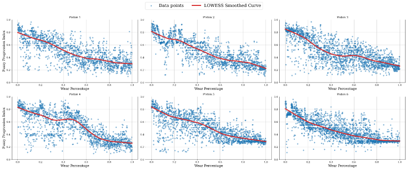
Using that fuzzy cluster results, the FPI values were generated for each engine block. Figure 6 shows the evolution of these FPI values (represented as points) generated by six pistons of the training set, and the LOWESS regression prediction for the pistons EOL.
5 A proposal for RUL estimation of the piston head
The values of LOWESS regression for each piston FPI have been valuable in determining the optimal number of clusters. However, due to its local nature, LOWESS regression is not a useful tool for predicting RUL outside of its training range, and it does not perform a reliable extrapolation outside of that training range. This was a major handicap for its online use, as the fitting is performed with the available parts, not with the complete curve.
To enhance the predictive capability of the previously calculated life trend, an additional step is proposed, consisting of the use of an exponential approximation. By fitting an exponential curve to the observed trend, using the number of clusters selected in the experiments described above, the approach aims to capture the underlying degradation dynamics in a smoother way. This method provides a compact mathematical representation of the FPI evolution, and facilitates the projection of future behavior.
5.1 A data-based model to predict the RUL from the Fuzzy Progression Index
To obtain an exponential data-based model, an exponential function for each piston in the training set was individually fit, and a threshold of this exponential function at the end of the lifetime was obtained. From these thresholds, the mean threshold and its variance were calculated. Next, the mean exponential function of the training set was computed. This was the function used as a model of the FPI in the testing phase. Subsequently, when evaluating the test set, a correction was applied to this mean exponential trend by incorporating the already observed residual values for each individually generated part and piston. This adjustment aims to refine the prediction by considering the previous piston behavior, which, in general, shows deviations that were not captured during the initial adjustment process. This adjustment improves the accuracy of the RUL estimation of the model through unobserved data.
5.2 Experimental results in the case study
Figure 7 presents the progressive estimation of the percentage of remaining parts for each of the test pistons at various points throughout their life cycle. The FPI value of each produced part is shown as a blue point, while the average trend for the exponential function derived from the training set is shown as a dotted red line. The dark blue line represents the corrected trend, obtained by adjusting the average exponential curve based on the residual values associated with each part for the current piston. Additionally, the orange and green vertical lines indicate the estimated range marking the end of the life cycle; specifically, these points correspond to the intersection of the corrected trend and the threshold value, considering both plus and minus one standard deviation. This visualization provides a clear and interpretable summary of the model’s performance, highlighting the variability inherent in the predictions and offering a practical estimation window for the remaining useful life of the components.
In particular, it is observed that each piston in the test set falls into one of the three possible estimation outcomes: underestimation, where the model predicts less remaining life than is actually present; overestimation, where the predicted remaining life exceeds the true value; and accurate prediction, where the estimation closely matches the actual remaining life. This variability highlights both the strengths and limitations of the proposed methodology, emphasizing the importance of understanding the conditions under which the model reliably performs versus when it tends to deviate. Such insights are critical for refining the approach and ensuring more consistent predictive performance across diverse operating scenarios.

In Table 2, the predicted threshold values for each chunk are presented, with the rows shaded in grey specifically highlighting the chunks that correspond to the actual EOL cycle for each piston in the test set.
| Piston | Chunk | Input Threshold | Output Threshold |
|---|---|---|---|
| 1 | 1 | 0.865 | 0.961 |
| 1 | 2 | 0.865 | 0.961 |
| 1 | 3 | 0.904 | 1.004 |
| 2 | 1 | 0.900 | 1.000 |
| 2 | 2 | 0.948 | 1.052 |
| 2 | 3 | 0.978 | 1.087 |
| 3 | 1 | 0.904 | 1.004 |
| 3 | 2 | 0.939 | 1.043 |
| 3 | 3 | 0.987 | 1.096 |
Figure 7 and table 2 shows that only the third piston EOL is included in the estimated interval, while piston 1 lasts an additional 18% on the predicted Upper Threshold, and piston 2 lasts about 9% under the Lower Threshold. However, it is not easy to interpret these results as under or over estimations for the RUL. The data used for training and testing were not obtained in a controlled environment where the maximum acceptable RUL was pursued. These data come from standard factory operation where pistons are changed on a preventive maintenance agenda, that requires changing the piston head after a fixed number of operations. Moreover, the number of performed operations usually changes due to other operational criteria, such as the convenience of performing a programmed stop to change the piston head, or the detection of anomalies after the injection stage.
Even with these caveats, the proposed approach is considered as a potential valuable tool for plant operators and managers, to perform predictive maintenance of the piston head.
6 Discussion and Conclusions
This work has developed a tool to estimate the Remaining Useful Life of the piston head in an injection machine.
The problem of estimating the RUL has been divided into two stages. First, to find a useful wear index, the Fuzzy Progression Indicator. Second, to use the actual index of each piston to predict the RUL.
The Fuzzy Progression Indicator is a first step for estimating the EOL and the RUL, thus being the bases for a predictive maintenance policy. This work has proposed to estimate the FPI in a three-stage data-driven methodology, that has been validated by experimental results. The first stage of the methodology builds a latent representation from the available data using a state-of-the-art autoencoder architecture, DCNN. The second stage requires a reduction of the latent space dimension. UMAP has been shown to be able to find a three-dimensional projection related to the piston wear and tear state. The third stage relies on fuzzy c-means to cluster the projected space, looking for overlapping regions that can be related to different wear states. The membership vector of a projected point to the set of clusters allowed to obtain an index that ideally moves from the value of , for a new piston, with the total number of clusters, to a value of 1, for a totally worn piston. However, this index shows high variance and cannot be directly used to estimate the RUL.
To estimate the RUL, this work proposed to fit an exponential average function to the data of the training set. This function smooths out the highly variable FPI while still providing an acceptable forecast of the RUL. The prediction of the exponential function is corrected with the residuals of the actual index for the piston, which takes care, to some degree, of the deviation observed in a new piston from the expected behavior.
Currently, piston maintenance is preventive, and the piston is replaced after a pre-set number of injection operations, except when the piston wears out or fails early. The capability to predict the Remaining Useful Life of the piston introduces two significant operational benefits. Firstly, if piston degradation is detected prior to reaching the currently defined injection cycle threshold, maintenance activities can be proactively scheduled. This action would avoid unplanned downtime, which according to plant personnel, typically results in at least 45 minutes of machine unavailability in the event of an unexpected piston replacement. In contrast, planned maintenance can be executed within approximately 15 minutes. This results in a net gain of 30 minutes of productive machine time. Secondly, by extending piston usage beyond the conservative pre-set injection limit, based on actual condition rather than fixed intervals, spare part consumption can be optimized. This approach contributes to a reduction in the lifecycle cost of the component by decreasing its amortization per injection cycle.
Although further research is still needed, the current results are considered acceptable by plant managers in the sense that a plant preventive maintenance policy based on this tool can be tested.
In the immediate future we plan to validate the approach with a new batch of production data, which will include hundreds of life cycles to train and test. We will then implement a formal scheme to manage uncertainty, potentially considering unscented Kalman filter or particle filtering techniques.
References
- [1] Gerardo Acosta, Carlos Alonso González, and Belarmino Pulido. Basic tasks for knowledge-based supervision in process control. Engineering Applications of Artificial Intelligence, 14(4):441–455, 2001.
- [2] Nagdev Amruthnath and Tarun Gupta. A research study on unsupervised machine learning algorithms for early fault detection in predictive maintenance. In 2018 5th International Conference on Industrial Engineering and Applications (ICIEA), pages 355–361, 2018. doi:10.1109/IEA.2018.8387124.
- [3] Vepa Atamuradov, Kamal Medjaher, Pierre Dersin, Benjamin Lamoureux, and Noureddine Zerhouni. Prognostics and health management for maintenance practitioners-review, implementation and tools evaluation. International Journal of Prognostics and Health Management, 8(3):1–31, 2017.
- [4] Piero Baraldi, Francesco Cadini, Francesca Mangili, and Enrico Zio. Model-based and data-driven prognostics under different available information. Probabilistic Engineering Mechanics, 32:66–79, 2013.
- [5] James C Bezdek. Pattern recognition with fuzzy objective function algorithms. Springer Science & Business Media, 2013.
- [6] William S. Cleveland. Robust locally weighted regression and smoothing scatterplots. Journal of the American Statistical Association, 74(368):829–836, 1979. doi:10.1080/01621459.1979.10481038.
- [7] Miguel Cubero, Diego Garcia-Alvarez, Luis Ignacio Jiménez, Daniel López Gómez, Belarmino Pulido, and Carlos Alonso González. Deep-learning clustering to assess the health state in a die-casting process in the automotive industry. In 6th "International Conference on Control and Fault-Tolerant Systems (SYSTOL)", 2025.
- [8] Matthew J Daigle and Kai Goebel. A model-based prognostics approach applied to pneumatic valves. International Journal of Prognostics and Health Management Volume 2 (color), 84, 2011.
- [9] David Garcia de Vicuña Lopez de Ciordia. Application of time-series clustering for Factory 4.0 (in Spanish). Master’s thesis, Escuela de Ingenieria Informatica de Valladolid, Universidad de Valladolid, July 2024. Supervisors: B. Pulido, C. Alonso-Gonzalez.
- [10] Alberto Diez-Olivan, Javier Del Ser, Diego Galar, and Basilio Sierra. Data fusion and machine learning for industrial prognosis: Trends and perspectives towards industry 4.0. Information Fusion, 50:92–111, 2019. doi:10.1016/J.INFFUS.2018.10.005.
- [11] J. Y. Franceschi, A. Dieuleveut, and M. Jaggi. Unsupervised scalable representation learning for multivariate time series. Advances in Neural Information Processing Systems, 32, 2019.
- [12] B. Lafabregue, J. Weber, P. Gançarski, and G. Forestier. End-to-end deep representation learning for time series clustering: a comparative study. Data Mining and Knowledge Discovery, 36(1):29–81, 2022. doi:10.1007/S10618-021-00796-Y.
- [13] Han Li, Wei Zhao, Yuxi Zhang, and Enrico Zio. Remaining useful life prediction using multi-scale deep convolutional neural network. Applied Soft Computing, 89:106113, 2020. doi:10.1016/J.ASOC.2020.106113.
- [14] Elizabeth Ann Maharaj, Pierpaolo D’Urso, and Jorge Caiado. Time series clustering and classification. Chapman and Hall/CRC, 2019.
- [15] Leland McInnes, John Healy, Nathaniel Saul, and Lucas Großberger. UMAP: uniform manifold approximation and projection. Journal of Open Source Software, 3(29):861, 2018. doi:10.21105/JOSS.00861.
- [16] Bojana Nikolic, Jelena Ignjatic, Suzic Nikola, Branislav Stevanov, Aleksandar Rikalovic, et al. Predictive manufacturing systems in industry 4.0: Trends, benefits and challenges. In Proceedings of 28th DAAAM International Symposium on Intelligent Manufacturing and Automation, pages 796–802. DAAAM International, Vienna, Austria, 2017.
- [17] Anibal Hernando Novo. Health state estimation for an injection machine using deep-learning (in Spanish). BSc thesis, Escuela de Ingenieria Informatica de Valladolid, Universidad de Valladolid, July 2025. Supervisors: D. Garcia, B. Pulido.
- [18] Enrique H Ruspini. Numerical methods for fuzzy clustering. Information Sciences, 2(3):319–350, 1970. doi:10.1016/S0020-0255(70)80056-1.
- [19] Girish Kumar Singh et al. Induction machine drive condition monitoring and diagnostic research – A survey. Electric Power Systems Research, 64(2):145–158, 2003.
- [20] George J Vachtsevanos, Frank Lewis, Michael Roemer, Andrew Hess, and Biqing Wu. Intelligent fault diagnosis and prognosis for engineering systems, volume 456. Wiley Online Library, 2006.
- [21] Laurens van der Maaten and Geoffrey Hinton. Visualizing data using t-SNE. Journal of Machine Learning Research, 9(11):2579–2605, 2008.
- [22] Z. Wang, W. Yan, and T. Oates. Time series classification from scratch with deep neural networks: A strong baseline. In 2017 International Joint Conference on Neural Networks (IJCNN), pages 1578–1585. IEEE, 2017.
- [23] Shu-Xin Zhou. The practical applications of industry 4.0 technology to a new plant for both manufacturing technique and manufacturing process in new product introduction. IEEE Access, 9:149218–149226, 2021. doi:10.1109/ACCESS.2021.3124373.
- [24] Enrico Zio. Prognostics and health management of industrial equipment. Diagnostics and prognostics of engineering systems: methods and techniques, pages 333–356, 2013.
- [25] Enrico Zio. Chapter 8 – Data-driven prognostics and health management (PHM) for predictive maintenance of industrial components and systems. In Curtis Lee Smith, Katya Le Blanc, and Diego Mandelli, editors, Risk-Informed Methods and Applications in Nuclear and Energy Engineering, pages 113–137. Academic Press, 2024.