Multi-Criteria Route Planning with Little Regret

Abstract
Multi-criteria route planning arises naturally in real-world navigation scenarios where users care about more than just one objective – such as minimizing travel time while also avoiding steep inclines or unpaved surfaces or toll routes. To capture the possible trade-offs between competing criteria, many algorithms compute the set of Pareto-optimal paths, which are paths that are not dominated by others with respect to the considered cost vectors. However, the number of Pareto-optimal paths can grow exponentially with the size of the input graph. This leads to significant computational overhead and results in large output sets that overwhelm users with too many alternatives. In this work, we present a technique based on the notion of regret minimization that efficiently filters the Pareto set during or after the search to a subset of specified size. Regret minimizing algorithms identify such a representative solution subset by considering how any possible user values any subset with respect to the objectives. We prove that regret-based filtering provides us with quality guarantees for the two main query types that are considered in the context of multi-criteria route planning, namely constrained shortest path queries and personalized path queries. Furthermore, we design a novel regret minimization algorithm that works for any number of criteria, is easy to implement and produces solutions with much smaller regret value than the most commonly used baseline algorithm. We carefully describe how to incorporate our regret minimization algorithm into existing route planning techniques to drastically reduce their running times and space consumption, while still returning paths that are close-to-optimal.
Keywords and phrases:
Pareto-optimality, Regret minimization, Contraction HierarchiesFunding:
Carina Truschel: Funded by the Deutsche Forschungsgemeinschaft (DFG, German Research Foundation) – Project-ID 251654672 – TRR 161.Copyright and License:
2012 ACM Subject Classification:
Theory of computation Data structures design and analysis ; Theory of computation Shortest pathsEditors:
Jonas Sauer and Marie SchmidtSeries and Publisher:
1 Introduction
In many real-world navigation tasks, the optimal route is not sufficiently defined by a single criterion. For example, cyclists might want to follow the shortest path in terms of distance but only if it does not include too many steep climbs. For electric vehicles, travel time might be a primary objective but limited energy consumption should also be taken into account. Furthermore, users might want to also consider criteria as road surface quality, curviness, or tolls among others. Multi-criteria route planning addresses these scenarios. Here, given a graph , the edge costs are -dimensional vectors , where, for example, encodes travel time, distance, gas or energy consumption, and so on. As for the one-dimensional case, the cost of a path in the graph is the summed cost of its traversed edges . A path dominates another path , if holds for all cost dimensions and . There are three main types of route planning queries that are of interest for a given input source-target-node pair :
-
Full Pareto Set (FPS). Compute the set of Pareto-optimal paths from to .
-
Constrained Shortest Path (CSP). Given budgets , compute the --path with minimum cost under the constraint that for we have .
-
Personalized Shortest Path (PSP). For a given input weight vector , compute the --path that minimizes the personalized path cost .
It is well known, that CSP and PSP solutions are always Pareto-optimal. Thus, given the FPS, the last two types of queries can easily be answered. However, the goal for CSP and PSP is usually to compute the respective path without having to explore all Pareto-optimal paths. While the CSP problem is known to be NP-hard, PSP can indeed be solved in polynomial time using Dijkstra’s algorithm on the personalized edge costs . In [11] computing FPS for multi-criteria shortest paths in time-dependent train networks is tackled. As an example for CSP, finding constrained shortest paths for electric vehicles considers the travel time while not exceeding a maximum number of recharging stops [22] or the energy consumption does not exceed the capacity of the battery [4]. However, preprocessing based techniques to accelerate PSP queries also store sets of Pareto-optimal paths between selected node pairs [14].
The main issue is that the number of Pareto-optimal solutions can become huge (even in the bi-criteria case) and thus oftentimes further filtering needs to be applied to make route planning algorithms efficient and to present a sensible selection of alternatives to the user. Different ideas were proposed in the literature to filter a given set of Pareto-optimal elements. The goal is to efficiently maintain a core of solutions that are still representative of the full set. One such method is to define a relaxation of the dominance criterion. In [17] a tailored relaxation was implemented to reduce the number of Pareto-optimal journeys in public transport planning. For bi-objective shortest path problems, [15] describe an interesting approach to approximate the Pareto frontier using pairs of paths and guarantees per objective. Filtering the Pareto set in multi-criteria public transit routing in [8] uses fuzzy logic to identify significant journeys. In [7] restricted Pareto sets are used to provide a subset of the full Pareto set which excludes outliers having undesirable trade-offs between the criteria. A general and quite powerful approach for dominance relaxation in two-dimensional sets was described in [21]. Here the idea is to enlarge the dominance area, which for strict dominance is simply the lower left quadrant of the point. The problem with existing methods is that most of them are tailored to the bi-criteria case. Furthermore, one has little control over the number of Pareto-optimal elements that survive the filtering process. It could still be too large or it might happen that almost all solutions are filtered out.
In this paper, we use the notion of regret as introduced in [18] to identify representative subsets of size , where can be chosen as desired. Given a set of -dimensional elements and a subset , a user’s regret measures their disappointment when they have to choose the best option according to their preferences from instead of . More formally, a user has a preference or utility function and the regret of the user with respect to is defined as . By definition, we have .111In case , we simply set . The regret of is defined by the most regretful user, that is . Typically, the set of users is the set of all functions in a given class, most commonly the class of all non-negative linear combinations, that is , where the weight vector describes the importance of each dimension for the user. Figure 1 illustrates these concepts.
Given , the optimization goal of regret minimization algorithms is to find the subset of size at most with smallest regret. Obviously, can be restricted to only contain Pareto-optimal points from , as a dominated point can never have a higher utility than the dominating point. Still, computing an optimal poses an NP-hard problem [5]. We present a novel heuristic that computes subsets with small regret very quickly. This allows to integrate regret minimization in many applications where finding a representative subset of solutions is a frequent task, including multi-criteria route planning in road networks. Indeed, we show that leveraging regret filtering allows to compute constrained or personalized paths significantly faster, while ensuring that the resulting path (set) comes with small regret.
1.1 Further Related Work
A multitude of algorithms and heuristics has been proposed for all three main query types for multi-criteria route planning mentioned above. A* variants tailored to bi-objective search (BOA*) or multi-objective search (MOA*) have been demonstrated to greatly reduce the search space compared to Pareto-Dijkstra for FPS and CSP queries [24, 2, 20]. Methods to approximate the Pareto frontier were described in [15, 30]. In [29], an anytime approach was introduced that discovers a subset of Pareto-optimal paths quickly and then adds new solutions over time. A recent overview of the development of multi-objective route planning is provided in [27].
Even more pronounced speed-ups can be achieved if preprocessing is applied to the input graph. In [28], query answering for bi-criteria FPS using a contraction hierarchy (CH) data structure was reported to be two orders of magnitude faster than with BOA*. CH was also successfully applied to accelerate CSP [23, 13] as well PSP queries [12]. In [16], it was shown that filtering dominated points can be the bottleneck in bi-criteria CH construction as well as query answering. There, faster methods were proposed to compute Pareto-optimal path sets. But if the final set size remains large, the approach might still be too slow in practice. In all of these preprocessing-based techniques, sets of Pareto-optimal paths are precomputed and stored between selected pairs of nodes. While [12] allows to obtain approximate query results faster by only considering a subset of stored solutions on query time, non of the techniques apply filtering during the preprocessing, which results in data structures of substantial size.
1.2 Contribution
We show how multi-criteria route planning can be integrated with regret minimization. Compared to existing filtering methods, regret-based filtering has the advantage that it works for an arbitrary number of objectives and provides the user with the power to decide how many Pareto-optimal solutions shall be maintained to not exceed memory or running time resources. We first prove new theoretical properties of regret minimizing sets that are crucial for their application to route planning. As one main result, we show that the regret value does not deteriorate if we concatenate paths and combine their (filtered) solutions. This is important for many preprocessing-based techniques, in which this operation frequently occurs, for example, in multi-criteria contraction hierarchies (CH).
We describe how to construct the CH data structure with regret-based filtering as part of the preprocessing step (and thus significantly reduced space consumption), such that CSP and PSP queries can be answered much faster but with almost no loss in solution quality. As computing the solution subset with smallest regret poses an NP-hard problem, we also propose a novel and very efficient divide & conquer heuristic to compute high-quality subsets. In our experimental evaluation, we demonstrate that our new heuristic significantly outperforms the prevailing algorithm in solution quality, with only a small increase in running time. Furthermore, we show that using this heuristic as a subroutine for multi-criteria route planning results in well-performing preprocessing and query algorithms, even for a large number of cost dimensions.
2 Regret-Based Route Planning
The main idea is to use regret minimizing subsets to combat the combinatorial explosion of Pareto-optimal paths that is often observed in multi-criteria route planning algorithms. Regret is normally defined with respect to users that want to maximize their utility functions . But in the context of route planning, users want to minimize their (perceived) path costs. Thus, we now redefine regret as follows , where now expresses a penalty function. We remark that all regret minimizing algorithms can easily be adapted to also work with this definition.
2.1 Theoretical Bounds
Next, we prove a crucial property of the regret measure, namely that it does not stack when we combine partial solutions. This allows us to guarantee a good output quality when integrating regret-based pruning into various route planning algorithms, even if they need to combine partial solutions frequently. To concisely phrase our result, we introduce the following notations: With we refer to the set of cost vectors of Pareto-optimal paths from to , and with to a subset with regret . For two sets of cost vectors , we use to denote the set of elements derived from pairwise addition.
Theorem 1.
Let and be path sets with regret and with respect to and , then the regret of the combined path set is upper bounded by .
Proof.
We use and to abbreviate the notation. Let be any user and their penalty function for paths with cost . Let denote the preferred path of in the full path set, and the best one in the subset. Further, we use and to denote the two subpaths of with . We have . With and , we know that there exist paths and with and , respectively. Thus, it follows that:
Accordingly, and therefore . As this inequality holds for all users , the theorem follows. Of course, if we apply further filtering to a set that already was the result of prior filtering, the regret value might increase.
Lemma 2.
Let be path sets with and regrets , then .
Proof.
For a user , let the preferred paths from be , respectively. It follows that and . Combining the two inequalities yields . Thus, and . As this upper bound applies for all users, the lemma follows. Below, we will present route planning algorithms that aim to produce concise path sets for a given --query that induce little regret with respect to the FPS . The impact on PSP and CSP queries is expressed in the following lemmas.
Lemma 3.
For a PSP query from to with weight vector , returning yields a -approximation with .
Proof.
Let be the path with smallest personalized cost for the weight vector . As the regret for a subset is defined by the most regretful user, we know that and thus . Rearranging this formula, we get . Accordingly, ensuring small regret automatically provides us with an approximation guarantee for PSP queries. The same is not possible for CSP queries, as here the user specifies hard constraints on the accumulated path costs in all but the first dimension. Thus, if we prune any solution from , the CSP query might become infeasible. However, we can determine an upper bound on the accumulated constraint violation which is sufficient to guarantee a feasible solution.
Lemma 4.
For a CSP query from to with bounds for which contains a feasible path , the set contains a path that obeys with .
Proof.
The universe of users that define the regret value contains all linear combinations of the cost dimensions. We now focus on . Using this weight vector, we have for any path . Accordingly, where holds by the feasibility of . The statement follows from applying the same rearrangement to the formula as in the proof of Lemma 3. We remark that for the bi-criteria case, feasible CSP queries can easily be guaranteed by always maintaining the solution with smallest cost in the second dimension in .
2.2 Regret Minimizing Contraction Hierarchies
Contraction hierarchies (CH) were shown to be a very powerful technique for accelerating bi- and multi-objective route planning queries [9, 13, 12, 28, 16, 6, 3].
In the CH preprocessing phase, nodes are ordered by a ranking function . Then, so called shortcut edges are inserted between nodes if and there exists at least one Pareto-optimal path from to that does not contain a node of rank higher than . The shortcut edge represents all such Pareto-optimal paths from to and thus gets assigned the respective set of cost vectors . To obtain this shortcut set efficiently, a bottom-up approach is used. For original edges , the set initially only contains the cost vector associated with that edge. Then the nodes are considered in the order implied by the ranking and are contracted one-by-one. In the contraction step for node , it is checked for all pairs of neighbors of whether encodes Pareto-optimal paths from to . If this is the case, a shortcut from to is added (if it not already exists) and is augmented with the relevant cost vectors from . Then, and its incident edges are temporarily deleted from the graph. Note that by construction it holds that after each contraction the Pareto-optimal path costs between the remaining nodes in the graph are the same as in the original graph. After all nodes have been contracted, all temporarily deleted nodes and edges are inserted back into the graph.
In the resulting CH-graph, queries are answered with a bi-directional run of the Pareto-Dijkstra algorithm (or a MOA* variant). Here, forward and backward search only relax edges incident to a node if . This significantly reduces the search space but can be proven to nevertheless ensure correct query answering. To not only obtain the cost vectors of Pareto-optimal paths but also the paths themselves, a cost vector stores references to and with . This allows to recursively unpack a path that contains shortcut edges to a path that consists solely of original edges.
The memory consumption of the CH graph and the query performance crucially depend on the number of shortcut edges and especially the sizes of the cost vector sets associated with them. A simple approach to reduce the set sizes is to apply regret-based filtering to all independently with some fixed size upper bound . By virtue of Theorem 1, the regret for the result of any FPS query is upper bounded by the maximum regret obtained for any shortcut. But if one is interested not only in the path costs but also the paths themselves, the approach is insufficient. This is because we can no longer guarantee that the path unpacking procedure is successful, as for with and either or (or both) could have been pruned from their respective sets. Therefore, we use the following bottom-up approach instead: We process the edges/shortcuts ordered by . For a shortcut we consider all pairs of edges with and construct as the union of . Then, we apply regret-based pruning to . In this way, we guarantee that each cost vector that remains in is represented by two cost vectors in and , respectively. Figure 2 demonstrates the difference of maintaining the Pareto-optimal cost vector sets versus applying regret-based pruning on the set of cost vectors with a fixed size .
2.3 Route Planning Queries with Little Regret
For PSP queries there is no need to apply label pruning on query time, as the personalized weight vector reduces the edge costs to scalar values of which only the minimum needs to be maintained. But for FPS and CSP queries, label sizes tend to become huge during the search. A simple way to integrate regret pruning into answering FPS queries is to apply it whenever forward and backward search meet in bi-directional search. For query answering with CH, bi-directional search is the standard and it is also used as a standalone to reduce query time and space consumption [2]. For a node with a forward label and a backward label , computing can be very time consuming if both sets are large. First applying regret-based pruning to both sets to reduce them to a size of , respectively, allows to restrict the number of relevant elements to inspect to . According to Theorem 1, the resulting regret is upper bounded by the maximum of the individual regrets.
However, we can also use regret pruning within the forward or backward (or in unidirectional) search as follows. Whenever a node label size exceeds a threshold , e.g. , we apply pruning to reduce the size back to and then only proceed with the reduced label. Here, the regret might increase as shown in Lemma 2. However, this approach allows us to limit the space consumption of a query to and the cost of an edge relaxation to .
3 Regret Minimization Algorithms
The regret minimizing set problem (RMS) was introduced by [18], inspired by the application of multi-criteria decision making. Presenting a huge set of possibilities to an agent is often infeasible. Therefore, the goal is to select a (small) subset of possible decisions that are representative for the whole set and only communicate those to the agent. The approach is also used for database compression. A recent survey by [25] provides an extensive overview of several aspects of the regret minimization problem.
In [5, 1], RMS was proven to be NP-hard for dimensions . Several heuristic and approximation algorithms were designed for RMS that work for arbitrary . The algorithm by [18] greedily adds points to the solution subset until reaching the specified output size. The point selection leverages linear programming. The GeoGreedy algorithm by [19] greedily derives a solution subset based on geometric computations. The Sphere algorithm by [26] relies on sampling utility functions in order to find points with high scores. Similarly, the HittingSet approach introduced by [1] samples utility functions and reduces the RMS problem to a hitting set problem based thereupon. [18] also introduce the Cube algorithm. It partitions the multi-dimensional space into hypercubes by constructing equally-sized intervals in the first dimensions. From each hypercube the point having the highest value in the last dimension is added to the solution subset. Thus, the Cube algorithm returns a subset of size at most and a regret ratio of at most . The running time of the Cube algorithm is in with the space consumption being in . As this algorithm is easy to implement, scales very well in , and comes with quality guarantees, it is applicable in practice.
3.1 Hierarchical Regret Minimization
We propose a novel hierarchical regret minimizing algorithm HRMS that produces representative subsets of size for arbitrary dimension . The divide and conquer approach partitions the input set into smaller subsets and applies any pre-existing regret minimizing algorithm on each of the subsets to obtain intermediate regret minimizing sets. These sets are then merged in a hierarchical manner until only the final regret minimizing set remains. The hierarchical regret minimizing algorithm allows for user-defined adjustments to its hierarchy in order to obtain desired trade-offs between running time and solution quality. Figure 3 illustrates the basic algorithmic concept. Algorithm 1 shows the respective pseudo-code.
Here, is supposed to return a subset of of size with (hopefully) small regret. In our implementation, we use the Cube algorithm [18] for this purpose, due to its simplicity and efficiency even for high dimensions. However, one could plug in any other RMS algorithm as well. is supposed to partition into subsets, and to merge two point sets into one and to reduce the resulting set to the desired size. We next discuss sensible implementations of these two important routines.
3.2 Partitioning and Merging
The goal of the Partition method is to break the input set down into sufficiently small subsets of roughly similar size for efficient processing. A very simple partitioning method, is to randomly assign points to each of the subsets. However, it is advantageous to partition the input set in such way that the smaller subsets cover continuous parts of the multi-dimensional space. A good partition with regards to the HRMS algorithm yields subsets containing points from the Pareto front i.e. non-dominated points together with dominated points. During the conquer phase of the algorithm we handle each subset separately and reduce the number of overall points during the merging phase. In the worst case, all Pareto-optimal points are in one subset. Then, during the conquer phase we would exclude many such points in favor of dominated points from other subsets. Thus, it is ideal to have Pareto-optimal points in each of the subsets to ensure that the RMS algorithm is able to retrieve all of them. Our idea to achieve this is to divide the input space into equally-sized wedges between the x- and y- axes and to assign points to the wedges they are contained in. This likely ensures that each of the wedges covers a wide range of point values and also includes some Pareto-optimal points.
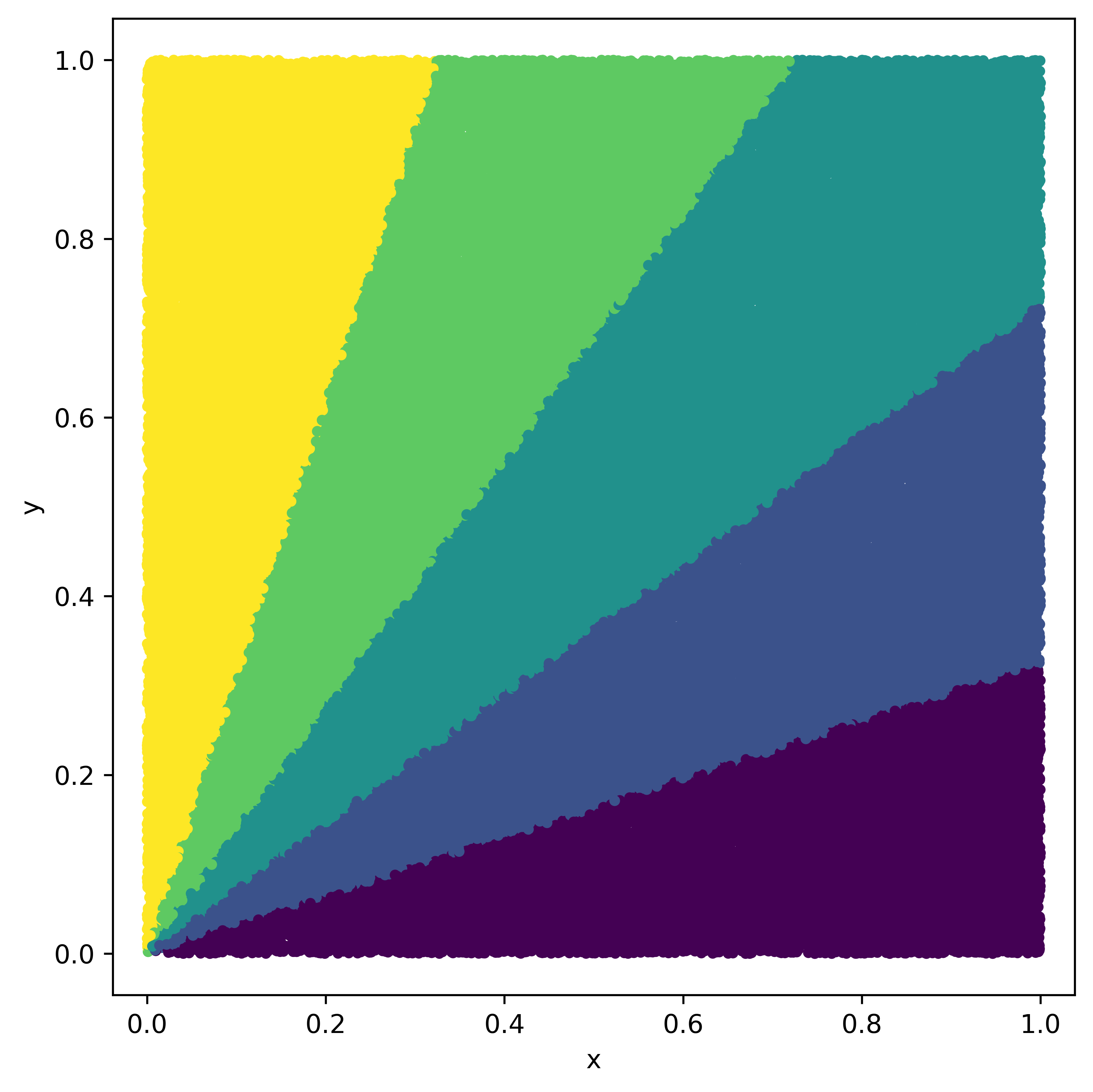
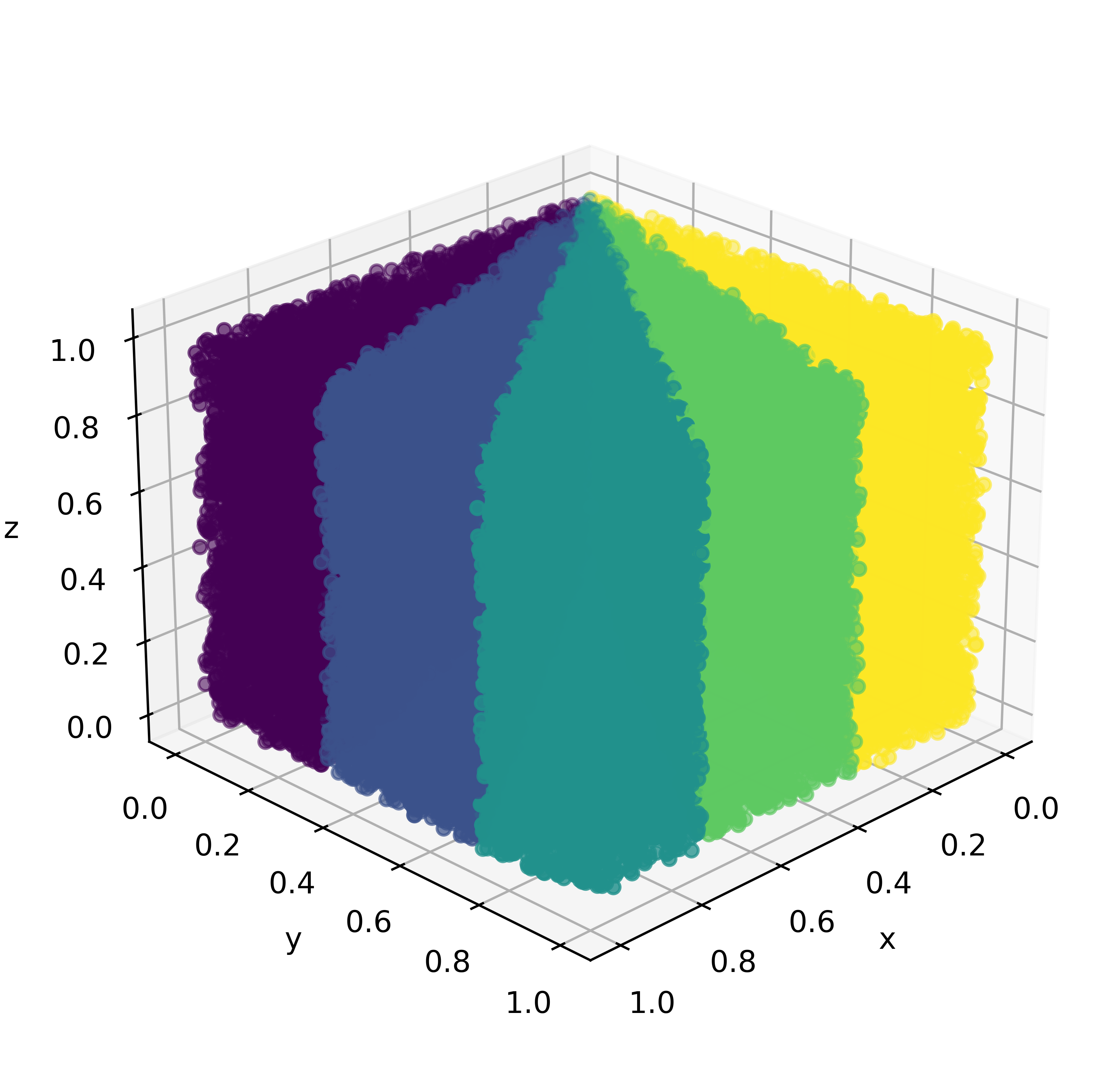
Figure 4 depicts an exemplarily partitioning of the input space in and dimensions.
The goal of the MERGE operation is to combine two point sets and but only keep the best points among them. A naive approach would again be to just randomly sample points from the union . However, this method is unlikely to produce good results. Since we already use an RMS algorithm to obtain the intermediate sets and , a natural way to merge would be to rerun said RMS algorithm on their union. In practice, this merging technique significantly increases the running time of the HRMS algorithm, though. A third method is to greedily remove points from the union until the desired output size is reached. Ideally, we would like to always select the point whose removal increases the regret the least. But computing the regret ratio requires to solve a linear program [18] and is thus also time intensive. As a compromise, we propose a sorted merge algorithm. It initially sorts and decreasingly in each of the dimensions. Then, the first points from the sets and corresponding to the decreasing order in the first dimension are retrieved. This procedure is repeated for each dimension to obtain the output set of given size. In this way, we select the promising points in each dimension.
3.3 Running Time Analysis
Considering the running time of the HRMS algorithm, we define as the running time required by the partitioning method, as the maximum running time of the chosen RMS algorithm executed on a subset , and be the running time of the chosen merging technique. With the partition method producing subsets, the total running time is in . Wedge-based partitioning takes . The Cube algorithm executed on a point subset with a desired output size of takes . Thus, the total time for processing all subsets is in . The merging calls take to go from subsets to subsets. Thus, the total merging time is in . As we have , we get an overall running time in which is close to the theoretical running time of the Cube algorithm. We will see that the two algorithms indeed also have similar practical running times, while HRMS produces sets with significantly smaller regret than Cube.
4 Experimental Evaluation
For regret minimizing set computation, we implemented the Cube and the HRMS algorithm in C++. Furthermore, we implemented the multi-objective CH approach with and without regret pruning, as well as the described query answering variants. Experiments were conducted on a single core of a 4.5 GHz AMD Ryzen 9 7950X 16-Core Processor with 188 GB of RAM.
4.1 Regret Minimization Results
First, we investigate the performance of our proposed HRMS algorithm and compare it to the Cube baseline. We chose the Cube algorithm since it scales well in arbitrary dimension and allows for a straightforward implementation. For our experiments, we use input sets consisting of points in dimensions and obtain subsets of size of . Generating the input sets is done by randomly sampling values from the uniform distribution in the range for each point. Running times and regret ratios are always averaged over 100 generated instances per tested value of .
In order to evaluate the solution quality of the HRMS algorithm, we need to obtain the regret of the solution subset which is defined by the most regretful user. To this end, we uniformly sample users represented by their weight vectors . We approximate the regret of the solution subset by computing the regret for each sampled user and extract the maximum among them. A similar approach is done in [1] by randomly sampling user weight vectors. We experimentally explore the effect of the sample size of users in the set on the resulting solution quality in Figure 5. Comparing sample sizes ranging from we conclude that the obtained regret ratios for the solution subsets are sufficiently similar among the sample sizes when ensuring that the extreme values and are represented at least once per dimension. Since computing the regret ratio for a given user weight vector involves traversing the entire input set , we use a sample size of to efficiently approximate the regret ratio for our experiments.
Prior to the experiments, we want to evaluate the geometric partitioning with respect to the resulting subset sizes and asses how close this angle-based partitioning comes to an ideal partitioning of the input space. The partitioning divides the input set into subsets based on the position of points in the -dimensional space. For the statistical assessment in Figure 6 input sizes of in dimensions and the output size and intermediate output size are used to obtain subsets. The value of is determined such that . Per tested value of , the partitioning described in Section 3.2 is executed on instances. Figure 6 reports on the average distribution of resulting subset sizes with the minimum, maximum and median size of subsets in the partition of the input set. Additionally, the number of subsets is also provided for each input size. An ideal partitioning yields equally-sized subsets each containing exactly points. This value depending on and is denoted as ideal (red markers).
The difference between the minimum and maximum subset sizes is fairly small considering input sets of up to 1 million points being divided into subsets. The smallest subsets contain 2 points and the largest 72 points. However, most observations in the distribution are much closer to the ideal subset size. The interquartile range for all input sizes always encloses the ideal subset size and the percentile is 12 points below the ideal value and the percentile is 20 points above the ideal value. Moreover, the median of actual subset sizes from the partitioning is within points of the ideal value. For the variation reduces to one point or less. The median is closer to the lower quartile value thus more subsets are slightly smaller than the median subset size.
Overall, the distribution of subset sizes is consistent throughout all input sizes. As the value of is equal for some input sizes e.g. , the ideal subset size varies, consequently shifting the box plots to a slightly higher subset size.
In conclusion, the geometric partitioning based on angles to the -axis produces subsets which are fairly equally-sized and close to the ideal subset size for a given value of . Further, the advantages of dividing the input space geometrically in contrast to a random partitioning prevail as the former ensures an even coverage of the Pareto-optimal points among the subsets.
Figure 7 compares the regret ratios of the HRMS algorithm using the geometric partitioning and the random partitioning. The former divides the input space into equally-sized wedges between the x- and y-axes whereas the latter divides the input set into subsets using the indices of points within the set. The solution quality resulting from the geometric partitioning is clearly preferable compared to the random partitioning. In dimensions, the improvement in regret ratio is up to a factor of on average to the random partitioning. The beneficial behavior of the geometric approach was observed consistently up to dimensions. Only for higher dimensions both versions of HRMS provide similar regret ratios. Thus, we conclude that the geometric partitioning is indeed preferred over the random partitioning in practice matching the previous theoretical considerations.
Considering the dimensional scalability of the HRMS algorithm, we use input sets of up to points in dimensions with the selection of being depicted in Figure 8 (running time) and Figure 9 (solution quality). For all tested dimensions, we observe the HRMS algorithm requiring slightly more time than the Cube algorithm executed directly on the input set which is in compliance with our theoretical analysis. However, as the number of dimensions increases, the practical running time of HRMS algorithm gets closer towards the running times of the Cube algorithm. In terms of the solution quality, the HRMS algorithm consistently outperforms the Cube algorithm by providing significantly lower regret ratios among all tested dimensions. The most significant improvement by the HRMS algorithm of up to a factor of on average is obtained in dimensions compared to Cube. In , and dimensions, the average improvement of HRMS compared to Cube is by factors of , and , respectively. However, the HRMS algorithm optimizes for objectives simultaneously and provides small representing subsets that still ensure that the most regretful user is about happy with the provided solution instead of the full alternatives in the input set. Hence, we conclude that the geometric partitioning together with the hierarchical merging of the HRMS algorithm is consistently advantageous in terms of the solution quality as opposed to the state-of-the-art algorithm Cube.
Further, we evaluate the ratio of Pareto-optimal points in the solution subsets of the HRMS algorithm compared to the Cube algorithm in Figure 10 for and dimensions and up to input points. In both dimensions, the HRMS algorithm retrieves more Pareto-optimal points in its output set than the Cube algorithm. More precisely, for two dimensions the HRMS provides a Pareto ratio of while the Cube only achieves . In three dimensions, the Pareto ratios are for the HRMS and for the Cube algorithm. Hence, the improvement in solution quality provided by the HRMS algorithm is due to retrieving more Pareto-optimal points from the input set than the Cube algorithm. During the partitioning phase we emphasize on dividing the input space in such way that each subset ideally contains a small fraction of the Pareto frontier. Further, the sorted merge during the hierarchical merging ensures to select points having high values in each of the dimensions which corresponds to the concept of Pareto-optimality.
We now want to evaluate the HRMS algorithm on input sets following different distributions which are closer to realistic input scenarios. To this end, we execute the algorithms on Gaussian distributed input sets. For the Gaussian generator, we sample values from the normal distribution with mean and standard deviation ensuring that all values are positive integers. The corresponding regret ratios for the HRMS algorithm are displayed in Figure 11. Again, the HRMS algorithm consistently produces lower regret ratios than the Cube algorithm on all tested dimensions up to . On average among the input sizes, we gain a maximal improvement factor of in dimensions compared to the Cube algorithm. Over all dimensions and input sizes, the average improvement of the HRMS algorithm is by a factor of .
4.2 Multi-Objective Route Planning Results
For studying the impact of regret-based filtering in multi-objective route planning, we used an established benchmark, namely the German road network with real cost dimensions222https://www.dropbox.com/s/tclrjdkfhabu27h/ger10.zip?dl=0 such as the distance, travel time, positive height difference and energy consumption for electric vehicles [12]. Each cost dimension was normalized to the interval . To study the scalability of the different methods, we selected cutouts with the number of nodes ranging from 10000 to 3 million.
4.2.1 Preprocessing
To allow for a fair comparison between classical multi-objective CH and our proposed variant with regret-based filtering, we first constructed a metric-independent CH-graph, also called Customizable Contraction Hierarchy (CCH) [10]. Here, shortcuts are assigned between all pairs of neighbors when a node is contracted. Afterwards, we use the described bottom-up procedure to equip the edges and shortcuts with sets of cost vectors that encode Pareto-optimal paths between their endpoints. We either use the mode full where we only filter dominated points, or the mode regret where we additionally use HRMS to reduce the cost vector size to at most . If not stated otherwise, we use .
In Table 1, the statistics of our benchmark instances are provided together with the experimental results for the first preprocessing step, namely the CCH construction. Note that we actually stop after contracting 99.7% of the nodes. Leaving this “core” of uncontracted nodes is a common method for multi-objective CH construction (see e.g. [12]), as the shortcuts introduced late in the process usually span large portions of the graph and thus usually also encode a huge number of Pareto-optimal paths. Preventing their insertion by stopping early helps to reduce the query time, although the query algorithm has to consider all nodes in the core. We observe that this preprocessing step is very fast and the number of shortcuts that are inserted is less than the number of original edges.
| properties | CCH | |||
|---|---|---|---|---|
| time | ||||
| RN1 | 10000 | 21498 | 17ms | 19958 |
| RN2 | 100000 | 214362 | 0.3s | 207900 |
| RN3 | 1000000 | 2125904 | 3.8s | 2070908 |
| RN4 | 3064263 | 6468394 | 20.2s | 6347312 |
In the second preprocessing step, the edge cost vectors are assigned. We set a timeout of 5 hours for this step. In Table 2, we see that for the full setting in which all Pareto-optimal solutions are maintained, we could only stay within that time limit for the graphs with up to 1 million nodes. While the average number of vectors per edge is not huge even for RN3, the maximum number grows quite severely. This not only consumes a lot of space but also increases the preprocessing time. Applying regret pruning, however, allows to perform this step very quickly on all networks as the number of vectors to process per shortcut is limited.
| CH full | CH regret | |||||
|---|---|---|---|---|---|---|
| time | avg | max | time | avg | max | |
| RN1 | 0.1s | 1.78 | 606 | 30ms | 1.19 | 5 |
| RN2 | 1.5m | 5.80 | 30709 | 0.4s | 1.23 | 5 |
| RN3 | 2.7h | 7.45 | 161260 | 4.2s | 1.22 | 5 |
| RN4 | - | - | - | 19.9s | 1.21 | 5 |
4.2.2 Personalized Shortest Path (PSP) queries
Having fewer cost vectors per shortcut also positively affects the query time, as fewer vectors need to be considered when relaxing an edge. We first evaluate PSP queries, where the user inputs source and target as well as a preference vector . We select 100 random source-target-pairs in each graph and choose different preference vectors for each pair: One random weight vector, one vector with all entries set to (that means, all dimensions are equally important) and the unit vectors. Therefore, in total we have 1200 test queries per graph in our setup with . As shown in Table 3, the running time of the Dijkstra baseline is in the order of seconds on the larger graphs. Using the full CH approach, query times are significantly reduced as only a small percentage of nodes and edges are considered on query time. But the acceleration also decreases steeply with increasing graph size, from around 940 for RN1 to around 45 for RN3. The main reason is that the average number of vectors that have to be relaxed per edge is quite large for RN3, which increases the query time. Using CH with regret filtering for every shortcut, that ratio is always upper bounded by . Note that the ratio of vectors per edge in a query comes indeed close to and is thus much larger than the average cost vector number per edge which is provided in Table 2. This is due to the fact that shortcuts between nodes with higher contraction rank are more likely to be considered on query time, but these are also the ones which tend to have the most cost vectors. Nevertheless, the cost vector size is drastically reduced compared to CH full and therefore the query answering stays fast even in the larger graphs, with a speed-up of over 600 for RN3 and RN4.
| Dijkstra | CH full | CH regret | |||
|---|---|---|---|---|---|
| time | time | ratio | time | ratio | |
| RN1 | 47ms | 0.05ms | 25.7 | 0.02ms | 3.6 |
| RN2 | 0.5s | 9.17ms | 196.1 | 0.20ms | 4.2 |
| RN3 | 5.3s | 0.12s | 257.3 | 8.14ms | 4.4 |
| RN4 | 17.6s | - | - | 28.59ms | 4.4 |
But of course the question is how the result quality is compromised by the regret-based filtering of the solutions. Over all instances, the observed maximum regret was at most 0.0613 and the average an order of magnitude smaller, namely around 0.0029. Thus, the obtained approximation factor (see Lemma 3) for PSP queries is upper bounded by 1.065 in our experiments, and on average solutions were within 2-3% of the optimal cost. This demonstrates that regret pruning allows to get close-to-optimal query results for PSP while significantly reducing the preprocessing and query time, as well as the space consumption.
To further shed light on the interplay of the dimension and the maximum number of cost vectors per shortcut, Table 4 shows regret values on the RN3 instance where cost vectors were created with entries u.a.r. in . We observe that the maximum regret stays small even if we only preserve vectors per shortcut. The average regret was again at least one order of magnitude smaller in all scenarios.
| 5 | 0.0409 | 0.0544 | 0.0204 |
|---|---|---|---|
| 10 | 0.0625 | 0.0572 | 0.0419 |
| 50 | 0.0638 | 0.0519 | 0.0481 |
| 100 | 0.0749 | 0.0495 | 0.0474 |
4.2.3 Constrained Shortest Path (CSP) queries
Finally, we investigate whether regret pruning is also useful in the context of CSP queries, where the user specifies upper bounds on all but the first cost dimension and aims at retrieving the path which obeys these bounds and has minimum cost in the first dimension. To construct sensible queries, we proceed as follows: We first select out of the available cost dimensions randomly. Then, for a source-target-pair, we compute the shortest path cost for all but the first cost dimension individually and set the bound for some . If not stated otherwise, we use . We consider the following query algorithms: Pareto-Dijkstra (PD), Pareto-Dijkstra with regret pruning (PDr), Pareto-CH-Dijkstra (PCHD) and Pareto-CH-Dijkstra with regret pruning (PCHDr). For the variants with regret pruning, we applied HRMS whenever the number of labels assigned to a node is equal to or exceeds to bring it back down to . We use in our experiments. Setting too low can actually be detrimental to faster query answering, as pruning too many labels might lead to additional operations if labels that dominate many others are removed. Thus, it is sensible to choose proportional to the dimension. Labels are pruned in all algorithms if a cost entry in any dimension exceeds the respective bound. Table 5 summarizes our findings on the RN1 and RN2 instances. In the 100 queries per experiment, we never observed that PD found a feasible solution but the regret-based variants did not. However, the costs in the first dimension were on average - larger than for the baseline. But this is a small increase compared to the large performance gain. For RN2 with larger and RN3 and RN4 the PD(r) baselines were too slow to conduct sufficiently many queries (single queries took hours). But PCHD(r) are applicable. For example, for RN4 and , query times for PCHD were in the order of several minutes, while PCHDr took at most 5 seconds.
| RN1 | RN2 | ||||
|---|---|---|---|---|---|
| PD | 25.0ms | 100.2ms | 2.7s | 2.1s | 22.0s |
| PDr | 22.1ms | 59.5ms | 0.5s | 0.8s | 2.7s |
| PCHD | 1.2ms | 13.0ms | 0.3s | 16.2ms | 57.3ms |
| PCHDr | 0.2ms | 0.4ms | 1.4ms | 1.3ms | 2.5ms |
5 Conclusions and Future Work
We demonstrated in this paper, that the regret-based pruning of multi-dimensional solution sets can be a very beneficial ingredient in multi-objective route planning, as it helps to significantly reduce query times and space consumption without having a severe impact on the solution quality. The efficiency of our new hierarchical algorithm for computing regret minimizing subsets, which produces solutions of high quality, is crucial in achieving these outcomes.
The proposed methods should be easy to integrate with existing heuristics for multi-objective search as MOA*. Nevertheless, it would be interesting to explore their interplay further and to apply methods as dimensionality reduction, used for faster dominance checks in MOA*, also for regret pruning.
References
- [1] Pankaj K. Agarwal, Nirman Kumar, Stavros Sintos, and Subhash Suri. Efficient Algorithms for k-Regret Minimizing Sets. In 16th International Symposium on Experimental Algorithms (SEA 2017), pages 7:1–7:23, 2017. doi:10.4230/LIPIcs.SEA.2017.7.
- [2] Saman Ahmadi, Guido Tack, Daniel D Harabor, and Philip Kilby. Bi-objective search with bi-directional A*. In Proceedings of the International Symposium on Combinatorial Search, volume 12, pages 142–144, 2021. doi:10.1609/socs.v12i1.18563.
- [3] Gernot Veit Batz and Peter Sanders. Time-dependent route planning with generalized objective functions. In European Symposium on Algorithms, pages 169–180. Springer, 2012. doi:10.1007/978-3-642-33090-2_16.
- [4] Moritz Baum, Julian Dibbelt, Dorothea Wagner, and Tobias Zündorf. Modeling and engineering constrained shortest path algorithms for battery electric vehicles. Transportation Science, 54(6):1571–1600, 2020. doi:10.1287/trsc.2020.0981.
- [5] Sean Chester, Alex Thomo, S. Venkatesh, and Sue Whitesides. Computing k-regret minimizing sets. Proceedings of the VLDB Endowment, 7(5):389–400, 2014. doi:10.14778/2732269.2732275.
- [6] Marek Cuchỳ, Jiří Vokřínek, and Michal Jakob. Multi-objective electric vehicle route and charging planning with contraction hierarchies. In Proceedings of the International Conference on Automated Planning and Scheduling, volume 34, pages 114–122, 2024. doi:10.1609/icaps.v34i1.31467.
- [7] Daniel Delling, Julian Dibbelt, and Thomas Pajor. Fast and exact public transit routing with restricted pareto sets. In 2019 Proceedings of the Twenty-First Workshop on Algorithm Engineering and Experiments (ALENEX), pages 54–65. SIAM, 2019. doi:10.1137/1.9781611975499.5.
- [8] Daniel Delling, Julian Dibbelt, Thomas Pajor, Dorothea Wagner, and Renato F Werneck. Computing multimodal journeys in practice. In International Symposium on Experimental Algorithms, pages 260–271. Springer, 2013. doi:10.1007/978-3-642-38527-8_24.
- [9] Daniel Delling and Dorothea Wagner. Pareto paths with sharc. In International Symposium on Experimental Algorithms, pages 125–136. Springer, 2009. doi:10.1007/978-3-642-02011-7_13.
- [10] Julian Dibbelt, Ben Strasser, and Dorothea Wagner. Customizable contraction hierarchies. Journal of Experimental Algorithmics (JEA), 21:1–49, 2016. doi:10.1145/2886843.
- [11] Yann Disser, Matthias Müller-Hannemann, and Mathias Schnee. Multi-criteria shortest paths in time-dependent train networks. In International Workshop on Experimental and Efficient Algorithms, pages 347–361. Springer, 2008. doi:10.1007/978-3-540-68552-4_26.
- [12] Stefan Funke, Sören Laue, and Sabine Storandt. Personal routes with high-dimensional costs and dynamic approximation guarantees. In 16th International Symposium on Experimental Algorithms (SEA 2017). Schloss-Dagstuhl-Leibniz Zentrum für Informatik, 2017. doi:10.4230/LIPIcs.SEA.2017.18.
- [13] Stefan Funke and Sabine Storandt. Polynomial-time construction of contraction hierarchies for multi-criteria objectives. In 2013 Proceedings of the Fifteenth Workshop on Algorithm Engineering and Experiments (ALENEX), pages 41–54. SIAM, 2013. doi:10.1137/1.9781611972931.4.
- [14] Stefan Funke and Sabine Storandt. Personalized route planning in road networks. In Proceedings of the 23rd SIGSPATIAL International Conference on Advances in Geographic Information Systems, pages 1–10, 2015. doi:10.1145/2820783.2820830.
- [15] Boris Goldin and Oren Salzman. Approximate bi-criteria search by efficient representation of subsets of the pareto-optimal frontier. In Proceedings of the International Conference on Automated Planning and Scheduling, volume 31, pages 149–158, 2021. doi:10.1609/icaps.v31i1.15957.
- [16] Demian Hespe, Peter Sanders, Sabine Storandt, and Carina Truschel. Pareto sums of pareto sets. In 31st Annual European Symposium on Algorithms (ESA 2023). Schloss-Dagstuhl-Leibniz Zentrum für Informatik, 2023. doi:10.4230/LIPIcs.ESA.2023.60.
- [17] Matthias Müller-Hannemann and Mathias Schnee. Finding all attractive train connections by multi-criteria pareto search. In Algorithmic Methods for Railway Optimization: International Dagstuhl Workshop, Dagstuhl Castle, Germany, June 20-25, 2004, 4th International Workshop, ATMOS 2004, Bergen, Norway, September 16-17, 2004, Revised Selected Papers, pages 246–263. Springer, 2007. doi:10.1007/978-3-540-74247-0_13.
- [18] Danupon Nanongkai, Atish Das Sarma, Ashwin Lall, Richard J Lipton, and Jun Xu. Regret-minimizing representative databases. Proceedings of the VLDB Endowment, 3(1-2):1114–1124, 2010. doi:10.14778/1920841.1920980.
- [19] Peng Peng and Raymond Chi-Wing Wong. Geometry approach for k-regret query. In IEEE 30th International Conference on Data Engineering (ICDE 2014), pages 772–783, 2014. doi:10.1109/ICDE.2014.6816699.
- [20] Zhongqiang Ren, Richard Zhan, Sivakumar Rathinam, Maxim Likhachev, and Howie Choset. Enhanced multi-objective A* using balanced binary search trees. In Proceedings of the international symposium on combinatorial search, volume 15, pages 162–170, 2022. doi:10.1609/socs.v15i1.21764.
- [21] Nicolás Rivera, Jorge A Baier, and Carlos Hernández. Subset approximation of pareto regions with bi-objective a. In Proceedings of the AAAI Conference on Artificial Intelligence, volume 36, pages 10345–10352, 2022. doi:10.1609/aaai.v36i9.21276.
- [22] Sabine Storandt. Quick and energy-efficient routes: computing constrained shortest paths for electric vehicles. In Proceedings of the 5th ACM SIGSPATIAL international workshop on computational transportation science, pages 20–25, 2012. doi:10.1145/2442942.2442947.
- [23] Sabine Storandt. Route planning for bicycles – exact constrained shortest paths made practical via contraction hierarchy. In Proceedings of the International Conference on Automated Planning and Scheduling, volume 22, pages 234–242, 2012. doi:10.1609/icaps.v22i1.13495.
- [24] Carlos Hernández Ulloa, William Yeoh, Jorge A Baier, Han Zhang, Luis Suazo, and Sven Koenig. A simple and fast bi-objective search algorithm. In Proceedings of the International Conference on Automated Planning and Scheduling, volume 30, pages 143–151, 2020. doi:10.1609/icaps.v30i1.6655.
- [25] Min Xie, Raymond Chi-Wing Wong, and Ashwin Lall. An experimental survey of regret minimization query and variants: bridging the best worlds between top-k query and skyline query. The VLDB Journal, 29(1):147–175, 2020. doi:10.1007/s00778-019-00570-z.
- [26] Min Xie, Raymond Chi-Wing Wong, Jian Li, Cheng Long, and Ashwin Lall. Efficient k-regret query algorithm with restriction-free bound for any dimensionality. In Proceedings of the 2018 International Conference on Management of Data, pages 959–974, 2018. doi:10.1145/3183713.3196903.
- [27] Mingzhou Yang, Ruolei Zeng, Arun Sharma, Shunichi Sawamura, William F Northrop, and Shashi Shekhar. Towards pareto-optimality with multi-level bi-objective routing: A summary of results. In Proceedings of the 17th ACM SIGSPATIAL International Workshop on Computational Transportation Science GenAI and Smart Mobility Session, pages 36–45, 2024. doi:10.1145/3681772.3698215.
- [28] Han Zhang, Oren Salzman, Ariel Felner, TK Satish Kumar, Carlos Hernández Ulloa, and Sven Koenig. Efficient multi-query bi-objective search via contraction hierarchies. In Proceedings of the International Conference on Automated Planning and Scheduling, volume 33, pages 452–461, 2023. doi:10.1609/icaps.v33i1.27225.
- [29] Han Zhang, Oren Salzman, Ariel Felner, Carlos Hernández Ulloa, and Sven Koenig. A*pex: Efficient anytime approximate multi-objective search. In Proceedings of the International Symposium on Combinatorial Search, volume 17, pages 179–187, 2024. doi:10.1609/socs.v17i1.31556.
- [30] Han Zhang, Oren Salzman, TK Satish Kumar, Ariel Felner, Carlos Hernández Ulloa, and Sven Koenig. A* pex: Efficient approximate multi-objective search on graphs. In Proceedings of the International Conference on Automated Planning and Scheduling, volume 32, pages 394–403, 2022. doi:10.1609/icaps.v32i1.19825.