Monitoring Latency on Submarine Cables: Limitations and Opportunities

Abstract
The world’s Submarine Cable Network (SCN) is a critical component of the Internet, supporting both inter- and intra- continental communication. We describe a methodology to extract packet latency (via RTT) information on submarine segments, using existing deployed infrastructure collecting standard traceroute measurements. The first component of the methodology identifies vantage points whose measurements traverse submarine segments. The second component provides novel, path-change-aware, approaches to extract the minRTT over the segments, using those vantage points. We demonstrate the efficacy of our method by using traceroute measurements from perfSONAR deployments as ground truth. Our results provide a clear view of the inherent limitations of existing deployed infrastructure. Although both our methodology and minimum RTT estimators raise the state of the art, they also reveal that such infrastructure cannot hope, in general, to access dynamic latency metrics such as latency variability (variance) arising from congestion.
Keywords and phrases:
Submarine Cable Network, Internet MeasurementCopyright and License:
![[Uncaptioned image]](x1.png) © Mia Weaver, Darryl Veitch, Paul Barford, Fabián E. Bustamante, and Esteban Carisimo; licensed under Creative Commons License CC-BY 4.0
© Mia Weaver, Darryl Veitch, Paul Barford, Fabián E. Bustamante, and Esteban Carisimo; licensed under Creative Commons License CC-BY 4.0
2012 ACM Subject Classification:
Networks Network measurementSupplementary Material:
Dataset: https://github.com/miaw-net/scn-dataarchived at
 swh:1:dir:5b0c37dc137bb8aae1140cdc2b0743ce0154385b
Acknowledgements:
The authors want to thank our shepherd Justine Sherry for her insights and thoughts on improvements that we were able to make in the paper. This work is supported by the National Science Foundation grants CNS-2107392, CNS-1703592, CNS-2039146, and CNS-2106517. Any opinions, findings, and conclusions or recommendations expressed in this material are those of the author(s) and do not necessarily reflect the views of the National Science Foundation. Darryl Veitch is partially supported by the Australian Research Council’s Discovery Projects funding scheme #DP230102856.Editors:
Katerina Argyraki and Aurojit PandaSeries and Publisher:
 Open Access Series in Informatics, Schloss Dagstuhl – Leibniz-Zentrum für Informatik
1 Introduction
Submarine cables are the foundation of global communications, enabling the vast majority of international data exchange and supporting the interconnectedness of economies, businesses, and societies. Monitoring and characterizing these critical systems is essential for optimizing their performance and ensuring effective network operations. The on-going build-out of submarine cable infrastructure and evolving network demands highlight the importance of studying how these systems respond to varying loads, environmental factors, and operational conditions [3, 24]. Insights into the dynamic properties of traffic on submarine cables can lead to improvements in network design, management practices, protocols and application performance, paving the way for more efficient and reliable global connectivity.
The question that drives this work is the following: what would it take to develop a cost effective capability for monitoring packet dynamics in the submarine cable network? Achieving such a capability presents significant technical challenges. Ideally, comprehensive packet monitoring capabilities (e.g., using specialized packet-capture systems) would be deployed at all ingress and egress points of submarine cables, allowing for real-time monitoring of packet latency, loss, jitter, etc. However, costs and the distributed, private ownership of submarine cable infrastructure make widespread deployment of such a capability a practical impossibility. An alternative approach involves leveraging existing measurement infrastructure to perform active probe-based monitoring. While this ameliorates cost and deployment concerns, it introduces its own set of challenges, including the need to identify strategically located vantage points to ensure comprehensive coverage, and determining how to extract meaningful information from measurement probes that traverse infrastructure that is physically distant from submarine cables and subject to different types of noise. In light of this, the more specific question we will address is the following: is it even feasible to use existing infrastructure to deliver dynamic measurement goals such as tracking latency variability?
In this paper we develop a methodology that we argue raises measurement capabilities to the point where they can meaningfully test the limits of existing measurement infrastructure for active probe-based submarine link monitoring. The methodology necessarily builds on a familiar active probing lineage, but introduces some unique features and perspective. We argue that the resulting approach is sufficiently powerful to merit the conclusion that existing measurement infrastructure is not capable of providing fine grained dynamic metrics, such as latency variability.
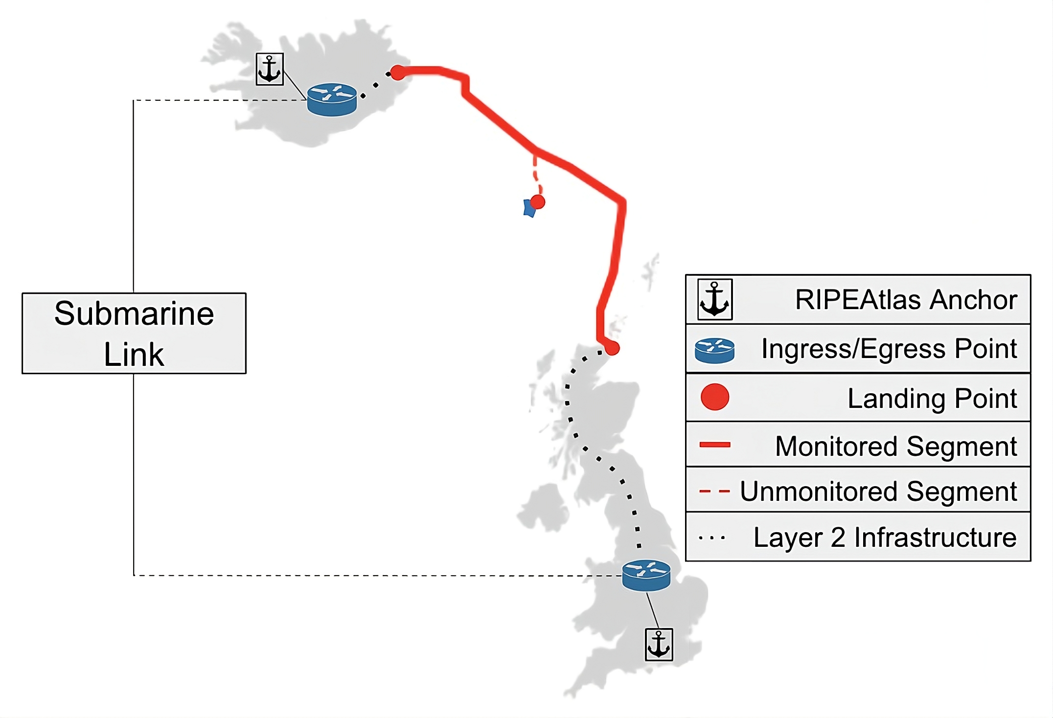
We define a Submarine Link (SL) as a layer 3 hop that includes a cable bundle that is deployed in a seabed that can span continents or two points on the same continent. An SL is delineated by two routers that respond to TTL-limited probes. These end points can be connected to infrastructure that does not respond to layer 3 probes but eventually leads to the landing points of the SL. Figure 1 illustrates this definition.
Our methodology leverages the availability of traceroute measurements collected from widely deployed vantage points (e.g., from RIPE Atlas [26] or Ark [4]). The first component of our methodology identifies vantage points that send traceroute probes that traverse SLs. Our method enables us to extract RTT measurements directed to layer 3 ingress/egress points of SLs, as illustrated in Figure 1. This component builds strongly on prior work [3, 24], yet requires significant enhancement to be adequate for our purposes here. We provide the background detail in Section 2, and enhancement details in Section 3.
The second component of our methodology is focused on extracting the Round Trip Time (RTT) over each identified SL, built from the raw RTTs from available traceroute measurements between identified vantage points. It does so in a novel way that properly addresses, for the first time, the inherent high impact issue of reverse path differences, both between participating measurements, and over the course of individual path measurements as they are made.
Our specific focus is the minimum round trip time (minRTT). While RTTs have long been recognised as a crucial measure of network conditions with direct implications to network health, SLA compliance and application performance [10, 21, 35, 30], there are good reasons to consider minRTT to be the most important RTT statistic. Accurate minRTT estimates are crucial to network protocols such as Google’s widely implemented congestion control algorithm, BBR [6], and play a central role in accurate network clock synchronization [5, 34]. They are used in latency-based network connectivity analysis [27, 28], and applications include use as a baseline for measuring congestion, and as input for both load balancing and provisioning decisions. Most importantly however, in particular for our purposes, it is the quantity that carries path change information, and this is what we must control if we hope to reliably isolate the portion of RTT belonging to an SL. This is because the minimum RTT of a link is a parameter that is not contingent upon network conditions and acts as a baseline. Any changes to this baseline indicate a change in the infrastructure being measured, not a change in traffic dynamics. As we explain in Section 2, this isolation is highly challenging due to the non-alignment of the underlying traceroute paths, complicated by “noise” contamination.
We develop two methods for identifying minRTT in our context. The first, unpaired estimation, is optimal in benign circumstances where the paths between probes sent to ingress compared to egress are maximally shared, but will suffer when these conditions are violated. The second, robust estimation, exploits traceroute probing structure and layers of non-linear filtering to generate an estimate far more robust to such effects, if (slightly) sub-optimal. It moreover leads to a highly robust form of minRTT timeseries visualisation, “”, of great utility. Details of each method are described in Section 5.
We demonstrate the efficacy of our minRTT estimation methods by comparing results with ground truth measurements on a selection of SLs that are directly monitored by perfSONAR nodes [22]. We confirm that the careful selection of vantage points results, as designed, in RTT measurements that are largely free of path changes that would otherwise greatly complicate extraction.
The contributions of the second component of our methodology are threefold:
-
i)
the methods themselves, which address path change issues in a principled way for the first time;
-
ii)
by comparing our minRTT result to those of a robust mean estimator, we are able to show how it is not feasible to extract more dynamic information, for example latency variances;
-
iii)
restricting to minRTT measurement, we exploit the ground truth to examine alternative approaches to the problem of how to blindly optimize the use of the multiple vantage points, and use it to justify a methodology to combine (minRTT) measurements across vantage points in a novel way.
We report on latency characteristics of all SLs that we can monitor during the month of December ‘24, highlighting the minRTTs that standard packet traffic are likely to encounter on these segments.
2 Background
In this section, we provide essential background by introducing the measurement platform that provides our traceroute data, defining the submarine links we aim to analyze, and outlining the key challenges inherent in this measurement process.
2.1 Measurement Data
RIPE Atlas is a widely-utilized measurement infrastructure hosting a global network of vantage points (anchors) that are used to launch active probe-based measurements [26]. The large number (approximately 800) of anchors distributed across different continents guarantees that some portion of the SCN will be traversed by ICMP-based traceroute mesh measurements between these anchors. We selected RIPE Atlas for SL monitoring not only due to this coverage, but also because of the publicly available repository of relatively frequent measurements that are launched in a full mesh between all anchors at a rate of one measurement every 15-minutes.
Given the availability of these consistent and geographically diverse measurements, we did not launch any additional measurements using RIPE Atlas. We focused instead on analyzing publicly available data.111For this we used the Python wrapper for the RIPE Atlas API [1]. While this design choice is somewhat restrictive, it facilitates reproducibility of our results, and is sufficient for our goals. Note that there is nothing about our methodology that is specific to RIPE Atlas. Our techniques can be directly applied to other similar datasets that are available from other widely-deployed measurement infrastructures, some of which are discussed below.
Despite the accessibility and geographic scope of RIPE Atlas infrastructure and measurement data, using it to monitor the SCN poses a significant challenge. RIPE Atlas anchors tend to be located in universities and laboratories geographically and topologically distant from SL ingress points and major Points of Presence (PoPs). Greater distance results in the possibility of greater measurement “noise” as discussed below. The geographic distribution also limits the conclusions one could offer on the SL network as a whole, however this is not an issue for this paper, which does not aim to provide a complete map of SLs, but rather to develop a methodology and use it to explore fundamental limitations for the SL monitoring problem.
Alternative Platforms.
Other platforms offer publicly available infrastructure that could be used to launch traceroute measurements, including Looking Glass Nodes (LGNs), CAIDA Archipelago (Ark), and perfSONAR. LGNs are routers made available by operators that can launch active probe-based measurements for the purpose of troubleshooting. In some cases LGNs may be located near submarine infrastructure, attractive for SL monitoring. However, LGNs do not provide tools to programmatically schedule measurements and often prohibit the use of automated scripts. Ark [4] offers constant, network-wide traceroute scans, enabling longitudinal studies of Internet-wide features. Ark is composed of approximately 280 nodes that conduct measurement campaigns to all /24 IPv4 prefixes announced in BGP routing tables. Ark’s measurement campaigns are relatively sparse in both time and space. The time between consecutive measurements of any given path is 24hrs in the best case, which limits its utility for monitoring dynamic properties of SLs. Finally, perfSONAR is a large scale platform with over 1000 instances deployed world wide, many of which are available for open testing of key measures of network performance [22].
Similar to RIPE Atlas, perfSONAR nodes are dedicated systems focused on end-to-end measurement. What is particularly compelling for our study is that through personal communications with ESnet [33], we were able to identify perfSONAR nodes deployed directly on routers connected on either side to 3 different submarine segments. By virtue of these deployments, we can assume measurements are very likely to be free of unshared path issues (see below), and we expect, and have verified, that they are free of level shifts associated with changes in layer 2. As such, data from these systems provided us with ground truth measurements of SL latency that we use in our study to assess the efficacy of our methodology. We utilize bidirectional measurements from the perfSONAR nodes on each side of a submarine segment to generate 6 ground truth measurement time series in total.
2.2 Submarine Cable Networks
Submarine cable systems form the backbone of global Internet connectivity, linking continents and enabling the high-capacity transmission of data across vast distances. A submarine cable system is often composed of multiple individual submarine segments, each connecting two specific endpoints along the cable’s route. These segments function as discrete physical links within the broader network, collectively forming the complete intercontinental pathway. Monitoring these individual segments provides insight into the performance and resilience of the entire submarine cable system.
To analyze the network-layer structure of these systems, we define a submarine link (SL) as the set of IP pairs extracted from consecutive traceroute hops traversing submarine segments in a single direction (see Figure 1), with a submarine segment monitored bidirectionally corresponding to two SLs. Submarine cable ingress and egress points are typically housed within facilities equipped with co-located routers that possess multiple ingress and egress interfaces. Consequently, multiple IP address pairs often correspond to the same underlying infrastructure. To geolocate these IP addresses, we utilize a combination of RTT measurements, geographic hints embedded in DNS records, and the Hoiho geolocation tool. The SCN infrastructure we seek to monitor lies between these identified near-side (ingress) and far-side (egress) IP addresses. We monitor conditions on 101 SLs.
2.3 Measurement Challenges
Ideally, we would like to instrument the SL with dedicated, time synchronized monitoring infrastructure at each end, to obtain a direct RTT timeseries measurement. Our task is to make the best possible estimate of the properties of this ideal timeseries by exploiting available traceroute measurements. It is not clear a priori which of its properties can be effectively extracted.
We list below a set of concerns inherent in traceroute-based measurement that create difficulties and limitations on what is achievable for our purposes [23]. Here we provide a brief general overview of these sources of “noise.” A more technical and detailed description is given in Section 5, where we develop methods to address them.
ICMP Packet Handling.
Routers treat ICMP packets differently from regular traffic, often processing them on a slower path through the router [23]. This overhead is an additional latency added to the reported RTT, effectively an error on top of the actual transit time of data packets traveling along the same route. Additionally, some traceroute probes may be subject to ICMP rate limiting on routers, wherein packets are routinely dropped. This reduces visibility into a network link and limits the amount of available data [11, 25].
Traceroute Implementation.
The implementation of traceroute on a given vantage point can introduce its own measurement overhead, adding an artificial delay that is independent of the network’s actual properties. This overhead is expected to remain relatively constant, however.
Congestion.
Measured RTTs combine latency components due to congestion at each hop. The longer the path, the more the cumulative, time varying congestion over the hops will complicate the extraction of the SL signal we seek. Even over short paths, high congestion levels can make extraction of target SL latency metrics very difficult.
Clock Errors.
Timing errors across measurement vantage points can introduce additional errors that may be hard to distinguish from other sources of noise.
Hidden Infrastructure.
Measurements over an SL combine variation due to network conditions on the cable itself with variation in the hidden layer 2 infrastructure that connects the submarine cable’s landing point to an inland PoP. Variability in this infrastructure, due to congestion or even path changes, could appear as level shifts or latency spikes that we may erroneously attribute to part of the measurement path outside of the SL.
Unshared Reverse Paths.
A fundamental limitation of traceroute is its inability to observe the reverse path from any given hop back to the source. The further the vantage point is from the SL, the greater the chance that the return paths from the ingress and egress routers back to it will be different. In that case, the hope of isolating the SL’s latency through, conceptually, “egressRTT - ingressRTT”, will be greatly impacted.
It is important not to confuse this problem with the well-known issue of asymmetry of the forward and reverse paths. In our context, asymmetry of the return is not a problem, what we require is that the return path for ingress and egress coincide (the MSP property of Section 5).
3 Vantage Point Selection
Mapping the paths of submarine cables requires a combination of curated infrastructure data, strategic vantage point and destination selection, and rigorous validation of measurement results. Given the challenges of observing SLs directly, our approach integrates publicly available cable system data with traceroute-based inference techniques.
We begin by constructing a detailed repository of over 350 submarine cable systems, capturing geographic locations, topological information, ownership, and known Autonomous System (AS) users to guide vantage point selection. Using this data, we identify network PoPs near cable landing stations and select RIPE Atlas vantage points positioned to provide optimal visibility into submarine segments. We search the measurements made from these vantage points to identify likely SL ingress/egress IP addresses. We were able to identify 423 unique ingress-egress IP pairs from 32 submarine cable systems that we could monitor. Over the course of our study, these IP addresses were remarkably stable, enabling consistent identification of RTT measurements to the ingress and egress of the SLs.
To confirm that a measurement indeed crosses its target SL, we apply a combination of geolocation analysis, speed-of-light constraints, and AS ownership validation, ensuring that observed links align with known submarine infrastructure. This enabled us to identify RIPE Atlas anchor (Origin, Destination) pairs that provided traceroute measurements used in our study. Within this dataset we identify 64 cable segments, 37 of which we monitor bidirectionally, yielding 101 unique traceroute data sets crossing SLs. This section describes our methodology, from data collection to validation, and outlines the criteria used to refine our set of vantage points.
3.1 Submarine Cable System Data Set
Positing that vantage points topologically and geographically near to submarine ingress points provide a more accurate view of cable behavior, we manually construct a knowledge base coalescing cable system landing point locations and information about known owners and users of specific submarine infrastructure. This repository includes details of geographic and topological information for over 350 submarine cable systems, which we use in vantage point selection, traceroute collection, and SL identification. We reference comprehensive submarine cable system maps hosted by Infrapedia and Telegeography, network maps provided by ISPs with major global footprints (i.e., Arelion, CenturyLink, and PCCW), industry reports, and cable system information provided by online data sets such as Submarine Network’s [12, 31, 32].
3.2 Methodology
To measure latency on a submarine segment, a vantage point(s) providing an accurate perspective, or as accurate a perspective as possible, is required. We first identify vantage points that meet the baseline criteria of launching measurements which cross the target submarine infrastructure and then filter for the highest quality candidates.
SL ingress points are typically situated at further inland network PoPs and data centers which connect to submarine cables via hidden layer 2 infrastructure (i.e., AEC-1 222This segment comprises AEC-1, CeltixConnect, and a terrestrial component over Ireland, as reported in [31]. Our ground truth measurements provided via ESnet report measurements over this combined infrastructure [33]. connects facilities Equinix LD6 in London and Equinix NY5 in New York City [31]). Because of this hidden layer-2 infrastructure, submarine links in traceroute measurements must be mapped to the major PoPs connected to the segment, and vantage points near these PoPs provide a better perspective of network behavior than those situated near the actual landing points (LPs).
We developed an approach to select RIPE Atlas anchors geographically near these PoPs, first extracting the latitude and longitude of LP cities using the python library GeoPy, then using iGDB to identify up to three PoPs in nearby major city centers [2, 14]. When identifying PoPs near an LP, we give priority to those used by known operators and users of the target submarine cable system. Next, we collect a set of candidate RIPE Atlas pairs wherein each node is within 100km of a PoP near the ingress or egress point of the target submarine segment. The purpose of using three nearby PoPs is to increase the number of candidate VPs meeting our baseline criteria. The remainder of our methodology seeks to reduce this set of VPs crossing a target SL to those that provide the highest quality data (i.e., lowest noise), so our key results are not sensitive to this threshold. We collect measurements between each pair from the pre-existing RIPE Atlas anchor mesh measurement repository rather than launching our own, user-defined measurements.
Following a similar methodology as proposed by Ramanathan et al. [24], we use a combination of IP geolocation, speed of light constraint RTT prediction, and AS identification to verify that a traceroute crosses the target submarine infrastructure. However, our methodology differs in that we identify vantage points specifically near SL ingress points, towards the goal of minimizing noise in the measurements.
Speed of Light Constraint.
We prune traceroutes which could not in fact have traversed the target submarine cable segment by comparing against a speed of light lower bound, following the methodology proposed in [29]. We ensure that the RTT is consistent with SL traversal, (i.e., is greater than the minimum implied by the great circle distance between the two LPs and the speed of light in fiber).
IP Geolocation.
When geolocating the IP endpoints of a potential SL, we begin by checking the RTTs associated with the ingress and egress IP addresses. If the RTT values indicate geographic proximity to a RIPE Atlas anchor, we infer the same city-level location. We selected a threshold of for matching ingress/egress IP address locations to RIPE Atlas anchor origin/destination locations, a value that identifies a sufficient number of reasonable vantage point candidates () for many SLs, from which our methodology can select a subset of highest quality candidate(s) (i.e., lowest noise). Since our methodology later filters out lower quality vantage points, it is only necessary to pick a threshold that will provide an initial set of candidates, and our results are not sensitive to this threshold.
Though this threshold ensures that SLs do have candidate vantage points in most cases, there are vantage points that, to be selected, would require a threshold large enough to potentially cause serious errors (i.e., mapping to incorrect underlying infrastructure). In such a case, we utilize Hoiho, an IP geolocation tool developed by Luckie et al., as utilized in iGDB and Nautilus [2, 15, 16, 24]. If Hoiho is unable to geolocate the IP endpoints, then we default to geographic pointers in DNS records and check for a match between the extracted city or airport code and target LP location. In the example provided in Listing 1, the ingress IP address is 0.54ms away from the origin located in Miami, Florida. The egress IP address is 1.3ms from the destination probe located in Fortaleza, Brazil. Thus, we confirm that the hop is crossing submarine infrastructure connecting Miami to Fortaleza. Cable system Monet has landing points in Boca Raton, Florida and Fortaleza; due to our mapping of PoPs to landing points, we infer that the SL ingress in Miami connects to the target segment of Monet.
AS Identification.
We verify that the ingress and/or egress IP address(es) of the SL is associated with an AS that is a known owner or user of the target submarine cable system. We use pointers in DNS records to identify AS ownership of the ingress and egress points of a SL. This step is used to differentiate cable segments with overlapping landing points.
Post-Processing.
Once we map a SL to the target infrastructure, we extract the pair used to generate the measurement and the IP addresses of the SL. For this study, we collect traceroutes between each pair over a month-long period, spanning from Dec. 1 to Dec. 31, 2024, and extract the RTTs associated with each end (ingress and egress) of the SL.
If during this longer time frame we see that the minimum RTT to the ingress point of the SL is 5.5ms, we exclude the vantage point. We do not impose this limit until the post-processing phase as when mapping traceroutes to underlying infrastructure, we consider only a single traceroute collected between a vantage point and destination, leaving the opportunity for congestion to temporarily inflate the ingress point RTT. The 5.5ms threshold was selected by hand to balance noise reduction, ensuring proximity to the ingress PoP, and enabling measurements from multiple RIPE nodes to be considered. Ideally, we match a submarine cable system to a set of at least 3 pairs that can be used to monitor the cable. Additionally, in the post-processing phase we manually remove pairs exhibiting any obvious erroneous data (i.e., change in RTT behavior resulting in values below the minimum possible RTT across the segment), or whose measurements only briefly cross the target infrastructure.
Limitations.
Multiple cable systems have identical ownership and nearby or overlapping landing points, introducing ambiguity into a subset of the identified SLs, particularly in traceroutes across cables connecting Eastern Asia or countries along the Suez Canal. Cable systems Apricot and APG, for example, both connect LPs near Tokyo to LPs in Singapore and are operated by NTT. In such cases, we are able to verify that submarine infrastructure is being crossed, and instead narrow down a set of potential cable systems. Future work could be done to further untangle these cable systems based on RTT values on the SL, as Apricot takes a longer path between Japan and Singapore than APG.
4 SCN Coverage
Our mapping effort identified 101 SLs 33337 submarine segments monitored bidrectionally, 27 submarine segments monitored unidirectionally: connecting all major regions of the world, with IP endpoints identified in 32 ASes (we are unable to map of the IP addresses we identified to an ASN), including tier-1 networks such as Arelion, CenturyLink, NTT, etc. Figure 2 shows a map of our coverage with SLs ranging in length from 130km to over 7000km. Details on all of these SLs can be found in the Appendix.
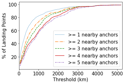
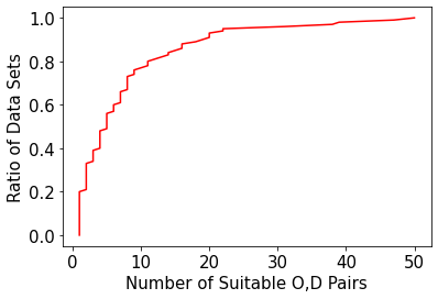
We found an average of 7.87 RIPE Atlas pairs per SL that are suitable for monitoring. Figure 3 shows a CDF of the number of suitable pairs identified per SL. Our coverage of the SCN in this study is limited by the fact that only of SCN landing points are within 1000km of five or more RIPE Atlas anchors, as shown in Figure 3, indicating that the set of suitable ensembles within a distance threshold of 100km to SL ingress/egress points is relatively small.
Please note: although we report on coverage, the goal of the work is not to provide a complete coverage of SLs.
Our vantage point selection methodology bears some similarity to Nautilus [24]. However, our objective differs significantly from Nautilus in that we seek to identify vantage points for the purpose of accurate monitoring of packet latency on submarine cables, rather than mapping SCN infrastructure itself. Despite Nautilus achieving wider coverage (mapping million IPv4 links to submarine infrastructure), we find that 86.8% of the 400+ unique SL IP endpoints identified via our methodology do not appear in the published Nautilus repository. We speculate that the difference in coverage is largely due to the fact that we select for vantage points within a limited distance to SCN landing points. This enables us to map traceroute hops to submarine infrastructure by using proximity between SL endpoints and RIPE Atlas anchors, even in the case of Hoiho failures and the absence of geographic pointers in DNS records. This technique is not used in Nautilus. Additionally, since Nautilus utilizes RIPE Atlas data from 2022, we suspect that some of the observed disparity is due in part to changes in infrastructure IP assignments during the 2 year period between our studies.
5 Latency Modeling and Estimation
Our fundamental approach to SL latency measurement is simple. We locate Origin and Destination probes that are close to Ingress and Egress routers to either side of the SL. By exploiting existing RTT measurements over using a that targets ingress, and by comparing with RTTs using over the path whose additional hop traverses the SL, we “subtract” to extract the SL component.
In practice there are many challenges, requiring a carefully constructed estimation procedure robust to path changes, failure of shared paths (see below), and congestion noise. In this section we formalise the above, describing the path model allowing link latency to be defined, isolated over the SL, and finally characterized.
5.1 Fundamentals
In this subsection we assume stable routing conditions. The RTT over any path (for fixed sized probe packets) can then be written as a constant minimum value corresponding to zero congestion, and a random congestion term. Thus,
| RTT over | |||
| RTT over | |||
| RTT over SL |
where , , are the minima, and , , the congestion terms.
In terms of available data, a single traceroute provides a trio of closely spaced measurements of , closely followed by a trio of measurements: . Thus a trace of traceroutes consists of measurements of each of and , organised temporally into trio-pairs. For (similarly for ) we label these in order as , , . Where measurements are missing (traceroute returns ), the missing elements are ignored.
To extract precise information on the SL from the measurements requires a critical assumption, that of maximally shared paths (MSP), meaning that the paths taken by packets sent to ingress and egress are identical in each direction, except for the SL itself. We illustrate the concept of MSP in Figure 4.
Assume MSP holds. Then the minima obey , and a natural unpaired estimator is
| (1) |
Under MSP the mean latency over the SL is also accessible. From the linearity of expectation a natural estimator is , where account for missing measurements. This is unbiased regardless of any correlations between congestion terms, including differing patterns or degree of missing measurements over the two routes.
5.2 Dealing with Path Changes
Path changes are endemic in the Internet, and result in sudden level shifts (LSes) in latency statistics. The upper left plot in Figure 5 provides an example where 2 LSes are seen in , and 3 in . The earliest and latest LSes match exactly, revealing that those changes occur on shared portions of the and paths, and so they cancel in the timeseries. The remaining LS is in only. Such an unshared LS induces a LS in - nominally impossible for an SL - proving in particular that MSP does not hold for this trace overall.
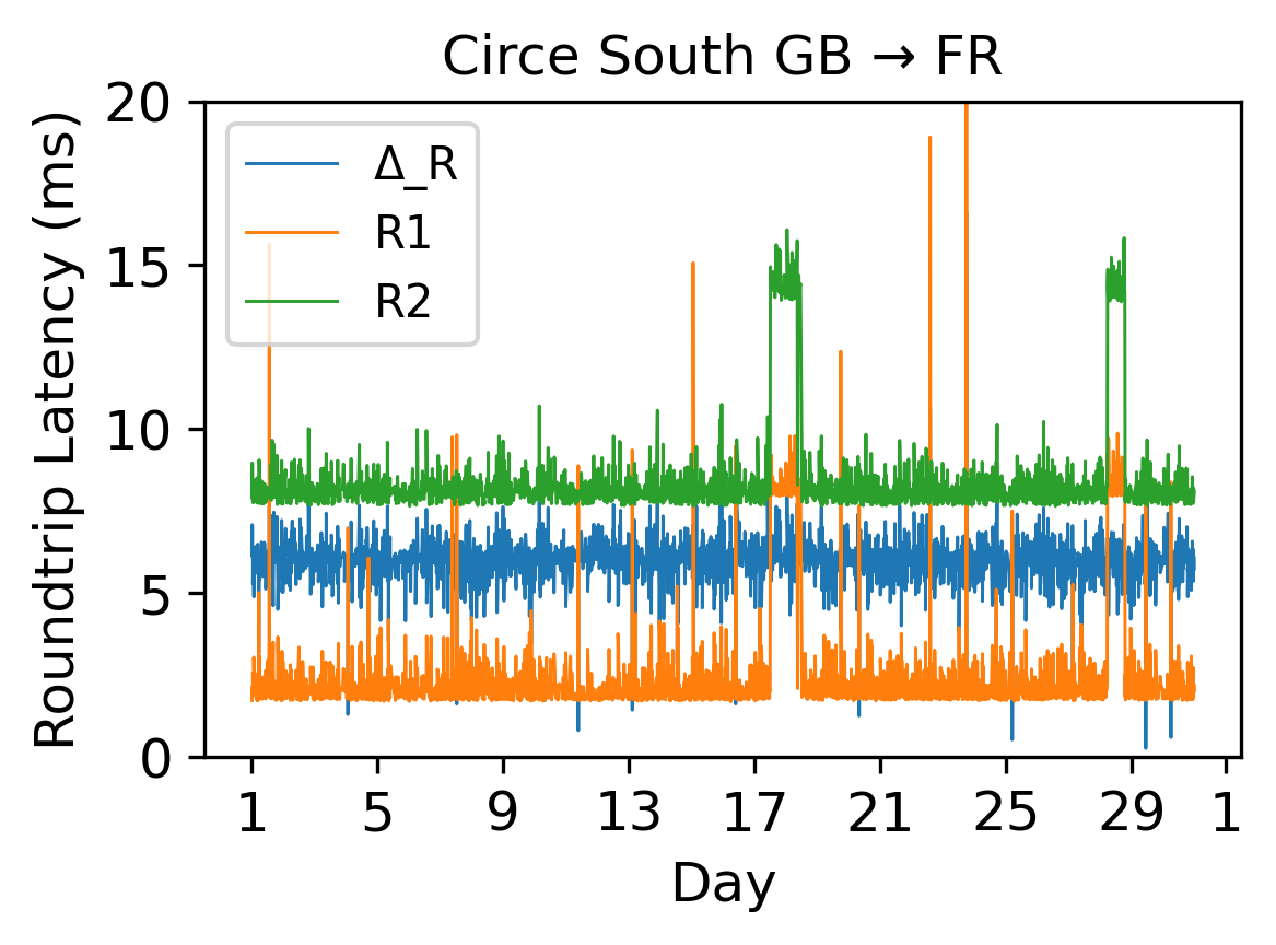
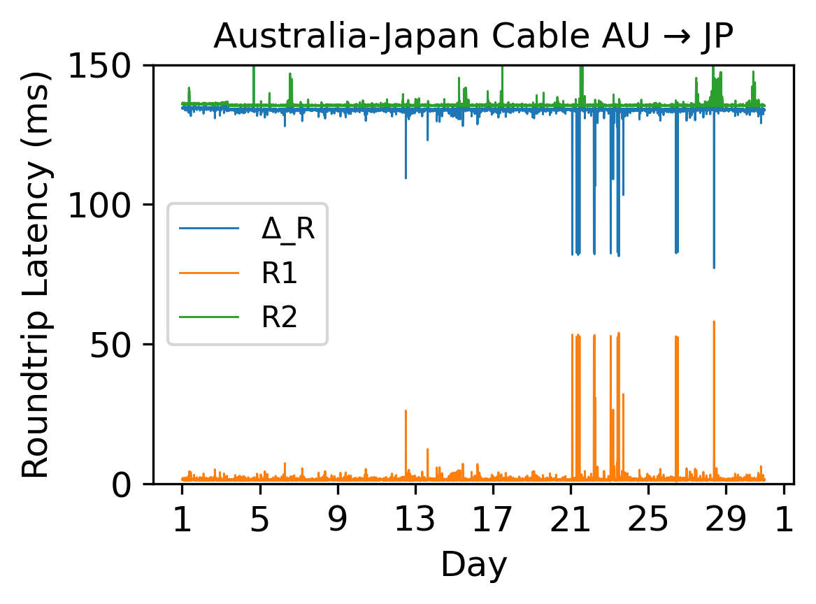
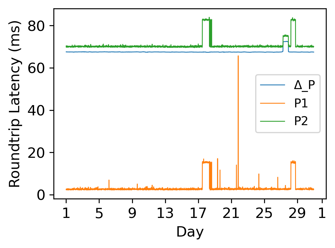
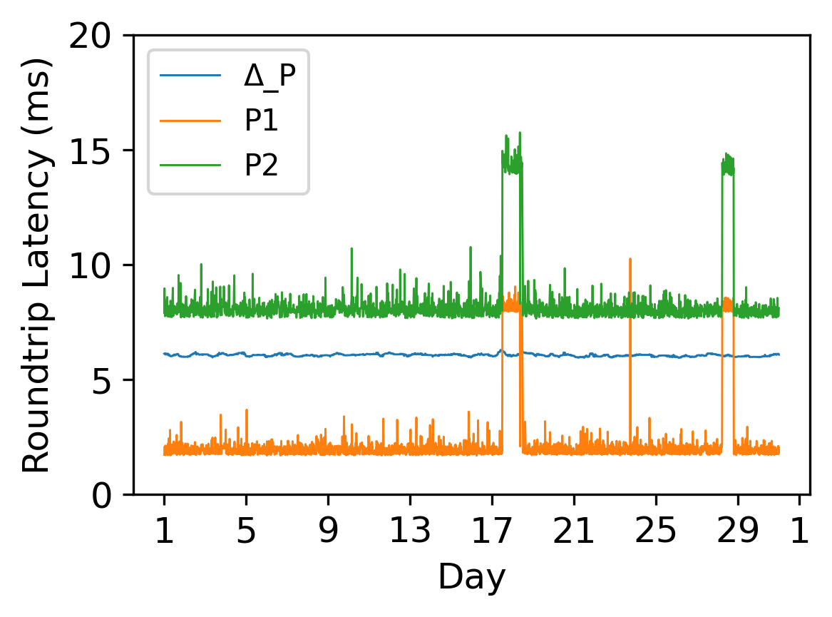
One of the limitations of the unpaired estimate (1) above is that it is not LS-aware - it sees only the lowest level in a multi-level data set, which results in unused samples at best, or completely erroneous estimates at worst. We now describe an improved approach to replace , leading to a robust .
We pre-process each trio-pair into a 2D timeseries , where is the min of the values in the trio, , , and similarly for . A sample is dropped when a trio is (). On the short intra-trio-pair timescale, path changes are very unlikely. Thus and will act as min-filtered versions of , over non-overlapping windows of width 3. This compresses values toward the , minima without distorting LS structure, so that the timeseries will still cancel shared LSes.
Consider again the noise about the underlying minima. Each measurement arises from a different packet, hence the samples of the congestion term for are all distinct from those of and so cannot cancel them, resulting in marked two-sided noise in . Being bidirectional, it cannot be suppressed using minimum-based filtering (to do so would lead to very significant errors, see Section 6.1). In the case of , the minimum filtering underlying significantly reduces the amplitude of the bidirectional noise. Just as importantly however, it also brings the minimum and median values closer together in each direction, so that the resulting noise in the difference is much more symmetrically centered. To augment this advantage we apply a sliding median filtering of window width to obtain (we use corresponding to hrs, see below). As this filter has the property that it preserves the position and amplitude of discontinuities, the result is effectively a form of timeseries that preserves unshared LSes (without the need for explicit detection), and enjoys low amplitude and locally symmetric noise over each level. The lower plot in Figure 5 shows , , and , the cleaner view compared to the upper plot on the same data, in particular with respect to , is striking. Further examples are provided in the center and right columns of Figure 5 where is free of LSes, so that is just the constant plus residual bidirectional noise that is approximately symmetric. When MSP holds this constant is simply , and the approximate symmetry motivates
| (2) |
This robust estimator avoids the inherent dangers of the unpaired estimator, which, being based on direct minima, is highly sensitive to anomalies of any kind (including many forms of clock error) even if very rare. The sliding median filtering also cleanly cancels very short lived LSes, which would not have provided adequate samples for estimation.
The clean view afforded by has another key advantage: it makes automatic segmentation into inter-LS zones with acceptable reliability feasible. We use the Python ruptures package for this purpose. To reduce the impact of errors in the inferred locations that nonetheless sometimes occur, for each returned zone we trim values from each end. Estimation is performed separately over each trimmed zone.
Window Size Sensitivity.
To assess the sensitivity of our results to the selected median filtering window size , we compute the excess kurtosis and skew over each level of the three exemplar data sets shown in Figure 5 as we vary the window size from to . We consider skew and excess kurtosis since the goal of our noise reduction method is to achieve a compact and symmetric distribution around the median for each level. A data set whose excess kurtosis and skew is near zero (for each level) is consistent with this goal. We find that the skew and absolute excess kurtosis values decrease dramatically as increases, finally trending towards zero beyond a certain value . However, after reaching a higher value , skew and excess kurtosis increase. This is because too large a window size discretizes the data into a small set of values, distorting moment based statistics like skew and kurtosis. We find that across the exemplars, the values of and vary, but that in all cases, is safely within the range . We conclude that is a relatively robust threshold, yielding skew values close to zero across the exemplar data sets without removing too many features from the data.
5.3 Dealing with MSP failure
Using the above methodology, for a given SL we obtain a set of timeseries , one per probe pair satisfying the careful VP selection described in Section 3. A timeseries with LSes gives rise to zones to be assessed, for a total of estimates capturing the different levels we see in the timeseries.
Careful examination against cases where we have ground truth (see below) failed to find any predictor enabling preferred level(s) to be identified. In fact even in the case of no LSes where , we have no way of confirming which obey MSP. As a result, we adopt a neutral approach and average estimates made using (2) to form
| (3) |
In the next section we will compare against an unpaired version of (3), that we define here as
| (4) |
which does not not require any LS segmentation to calculate.
When it comes to ground truth data, we use for visualization, but the unpaired estimator (1), as the robustness imperative is much reduced. In such a case the fact that the unpaired estimator directly targets minima (hence robust to congestion), does not suffer from any errors in LS segmentation, and makes use of all of the data, makes it preferable to (2).
To neutrally characterise the spread of available level estimates, we define the min-latency variability as
| (5) |
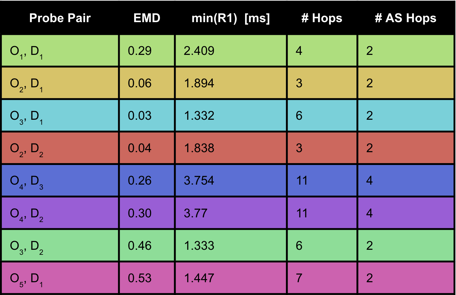
Figure 6 provides examples of all timeseries available for four SLs where ground truth data was available. Each case provides counter-examples to otherwise tempting principles we had hoped to propose as a basis for selecting the best level(s), and in particular those obeying MSP.
In the top plot many levels are close to 67ms, however the ground truth is elsewhere: a clustering heuristic would fail here. In the second plot the highest (purple) curve enjoys the smallest AS hop count of 2 compared to the other levels. Here routing might be expected to be more efficient and hence more likely to obey MSP, however it is the furthest from the ground truth. The third plot tells a similar tale for Origin probes (thick green and yellow curves at the top) that are closest to ingress in networking terms (smallest ), limiting the scope for routing diversity. Again they are actually the furthest from the ground truth. The last plot is paired with Table 1 supplying values of potential predictive criteria for each case, together with a measure of closeness to ground truth via Earth Mover Distance (EMD). No simple rule emerges. For example, pairs and are equal best with respect to network closeness and #AS hops, yet one is close to the ground truth and the other is not. Finally, collectively the examples show that the lowest level is not necessarily the best, contradicting the minimum based intuition focused on congestion.
5.4 Infeasibility of dynamic measurement
In ground truth data, where MSP holds, estimates of the (unshared) mean estimator and were typically found to be so close as to be practically indistinguishable (invisible in plots if we tried to show them). This is why, in the above, we have focussed on the minimum only. The immediate implication is that the standard deviation of RTT over SLs would be exceedingly hard to measure as it would lie under measurement uncertainty. However the implications of this finding are even more serious. It means that the difference is negligible compared to the spread of the levels observed when MSP does not hold, as we saw in detail in the previous subsection. Thus, as long as the MSP problem is not fully mastered, it is pointless to imagine we can “split the levels” to assess variance, or anything finer grained, with data of this type.
6 Results
In Section 5, we use a series of examples of traceroute measurements targeting SLs from identified vantage points to highlight the rationale and development of our methods for minRTT estimation. In what follows we now apply these techniques to all the SLs our methodology can reach given our data. Although longer data sets are available from RIPE Atlas, we restrict ourselves here to an analysis based on one month’s worth of data: December 2024.
In Section 6.1 we focus on cases where our perfSONAR ground truth is available, enabling a performance comparison of our minRTT estimators, to which we add a comparison against an additional naive estimator. Section 6.2 presents a summary of our findings over all SLs. Table 3 in the Appendix provides detailed data on all SLs, bolded rows corresponding to cases with available ground truth.
6.1 SLs with Ground Truth Measurements
There are six SLs where ground truth (GT) measurements are available, thanks to perfSONAR nodes deployed directly on ingress routers. A summary of these SLs and the number of pairs that monitor them is provided in Table 2 and in the Appendix. The number of pairs with measurements that traverse these SLs ranges from 4 to 12.
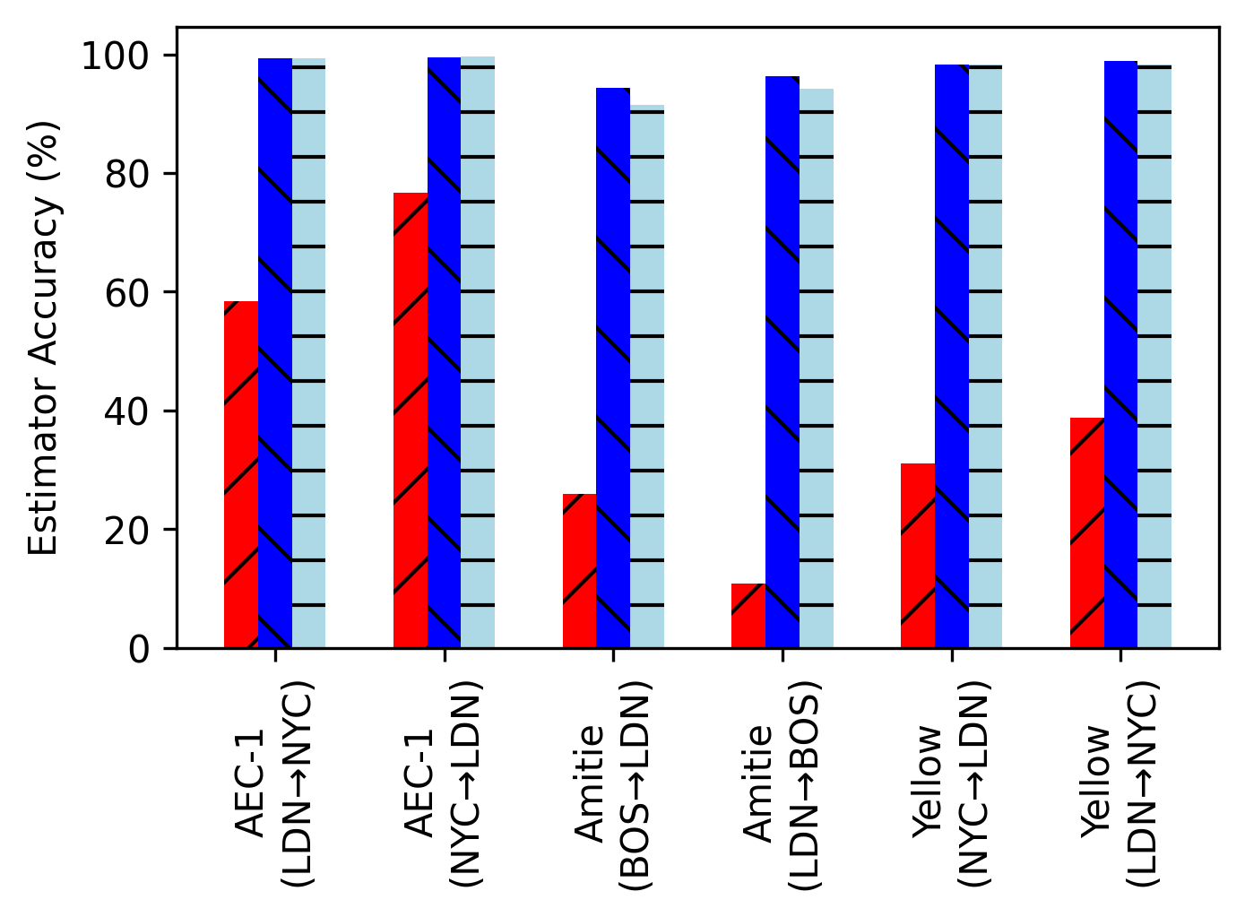
For these GT cases, in addition to our usual estimates based on RIPE Atlas traceroutes, we also calculate GT estimates according to (1), as described in the previous section. The performance of our estimates compared to the GT value is presented in Figure 8 in both relative (left plot as an accuracy) and absolute (center and right plots as an error in [ms]) terms.
| Cable Name | Segment | r̂SLu (ms) | r̂SL (ms) | GTr̂SL (ms) |
|---|---|---|---|---|
| aec-1 | Holyhead, GB Shirley, NY, US | 69.04 | 69.02 | 69.50 |
| aec-1 | Shirley, NY, US Holyhead, GB | 68.66 | 68.78 | 69.00 |
| amitie | Lynn, MA, US Bude, GB | 66.95 | 68.76 | 63.40 |
| amitie | Bude, GB Lynn, MA, US | 65.77 | 67.05 | 63.40 |
| yellow | Bellport, NY, US Bude, GB | 68.95 | 69.01 | 67.80 |
| yellow | Bude, GB Bellport, NY, US | 68.58 | 68.95 | 67.80 |
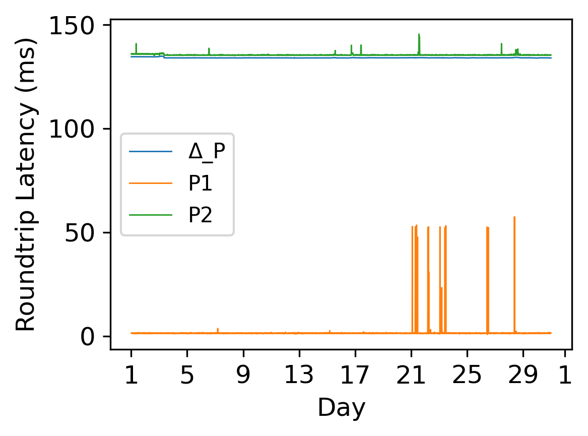
To provide some perspective on the importance of careful estimator design, in the left plot in Figure 8 we add results for a third naive estimator, corresponding to (4) with replaced by , where subtracting before taking the minimum is a fatal mismatch to the bidirectional nature of the noise. A visualization of this phenomenon is shown in Figure 7.
Both the unpaired and robust estimators generate values that are within 9.5% of the ground truth, which improves on the naive estimate by between 40% and 88%. As the result is so poor for the naive estimator, we drop any further comparisons with it.
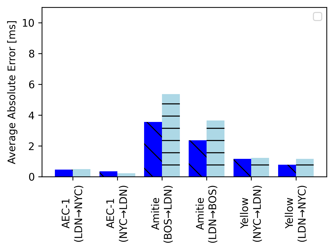
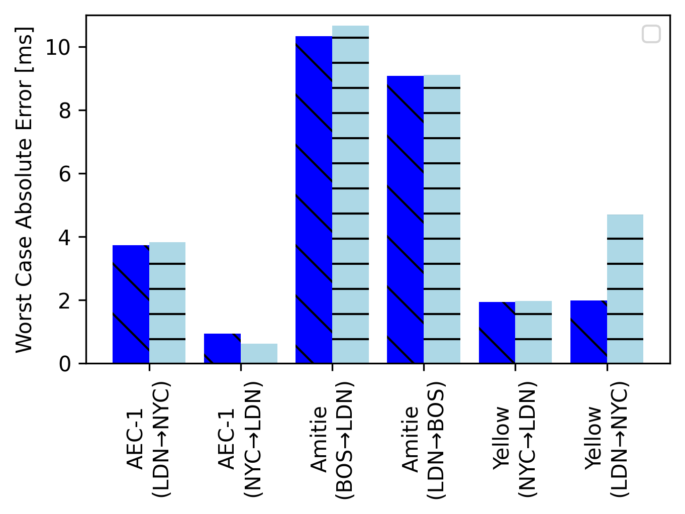
The central plot gives the same results reconfigured as average absolute error. As can be seen, the average error in each case is less than 5ms. The right hand plot isolates the worse of the individual (in the robust case) or (in the unpaired case) estimates available to form a worse case comparison. We see the worst case is only about twice the size of the average case. It is up to 10ms on SLs that have minRTTs on the order of 65ms.
Our view on these results is that given that the ground truth itself is not perfect (due to ICMP packet handling issues and others noises that could be responsible for much of the difference in level between different estimates), that our two estimators have comparable performance.
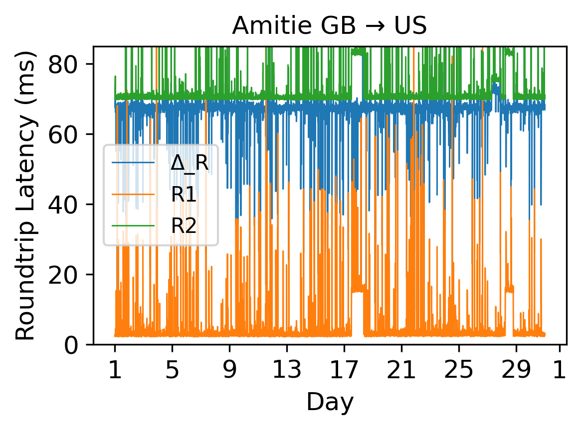
The relative improvement in the robust estimator in the worse-case compared to average results is consistent with its robust character. To expand on this, Figure 9 gives a specific example where the unpaired estimate , which focusses on the lower level after the LS, is worse than which averages the two levels, because the ground truth estimate is aligned with the upper level at .
6.2 SLs without Ground Truth
There are a total of 95 SLs that we can measure via RIPE Atlas for which we have no ground truth. We expect this to be by far the most common case in the future so it’s important to carefully consider the values that are reported and assess them relative to what we see in other measurements (including those with ground truth).
We provide details on all of the SLs that we can monitor in Table 3 in the Appendix. As illustrated in Figure 2, we find that our method applied to RIPE Atlas data identifies SLs with landing points on all continents (except Antartica) and with diverse deployment characteristics all over the world. Among all of these, there is relatively high coverage of transatlantic cable infrastructure (21 SLs monitored), which is a reflection of the dense deployment of RIPE Atlas nodes in Europe and the US. Transpacific coverage is also well represented in our data (13 SLs monitored). The remainder of the SLs are primarily intra-european and intra-asian. Perhaps not surprisingly due to the lack of RIPE Atlas nodes in these areas, coverage along the South American and African coasts is quite sparse, as is coverage of Oceania.
Examining the details of measurement coverage, we find two SLs (both transpacific) with 19 vantage points and up to 50 pair paths that traverse these. This is explained by the dense deployment of RIPE Atlas nodes on the California coast of the US. On average, there are about 8 pair paths that traverse SLs in our data. This means that in most cases, there is good measurement coverage on links that can be monitored. However, in the most limited cases, there is a single pair that can be used for monitoring – we find this to be the case on 21 of the SLs. While not inherently problematic, this does limit our ability to generate MLV values for those SLs. In closer examination of the RIPE Atlas data, this is due to our constraint of only selecting as vantage points anchors that are within 5.5ms of the ingress of the SL.
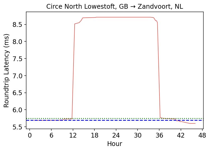
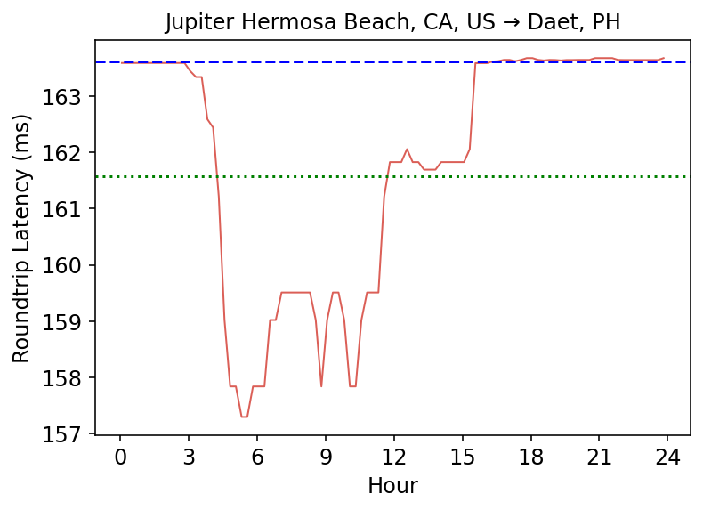
The values that we identify for minRTT range between about 5ms (e.g., the Circe North cable [18] between Zandvoort, NL and Lowestoft, GB shown in Figure 10), and 170ms (e.g., the Jupiter cable [19] between Daet, PH and Hermosa Beach, CA, US shown in Figure 10). We generally find a close correspondence between our unpaired and robust estimators for minRTT (less than 5ms difference) and manual checks with cable lengths indicate that the measurements are consistent with speed of light-based estimates [29]. This can be interpreted as indicating that most of these SLs have minimal noise profiles. However, in some instances, we find a somewhat significant difference. For example, on the Atlantic Crossing 1 cable [17] between Brookhaven, NY, US and Whitesands Bay, GB our unpaired estimator reports 66ms while the robust estimator reports 81ms. This SL like others with some disparity tend to appear on SLs where there is a single pair. In these cases, it’s impossible to generate an MLV to provide wider context.
Finally, turning our attention to MLV, these values vary widely over the monitored SLs. In general, they tend to be less than 10ms indicating a close correspondence in the timeseries of minRTT estimates from our robust estimator. This is a strong indicator of low noise on these SLs. Relatively higher MLV values (e.g., on the Pacific Crossing infrastructure [20], which includes MLVs of between 18ms and 73ms) indicate high levels of noise in timeseries of minRTT estimates and point to our robust estimator as a better predictor of minRTT.
7 Related Work
Our research builds on a substantial body of literature focused on measuring Internet links, with particular attention to underwater infrastructure.
The submarine cable network has been the focus of several recent empirical studies. Bischof et al. [3] underscored the critical role of the SCN by illustrating multiple cable failures and their cascading effects on global communication. Fanou et al. [9] examined the influence of a newly deployed cable in the South Atlantic on African nations, highlighting the socioeconomic impacts of SCN infrastructure. Liu et al. [13] demonstrated that many popular websites rely on SCN infrastructure for hosting objects, emphasizing the dependency of key Internet services on these undersea networks.
More recently, Carisimo et al. [7] explored the long-haul link network of the Internet, revealing that numerous intercontinental links terminate at inland locations thousands of kilometers from submarine landing sites. Ramanathan [24] introduced Nautilus, the first system designed to identify IP addresses likely to be associated with end points of submarine cables and map them to specific submarine cables. Nautilus employs proximity-based heuristics on intermediary traceroute hops, searching up to 1,000 km from a router’s geolocation in 50 km increments to associate network ingress and egress points with nearby cable landing stations. This differs from our proximity-based geolocation utilizing anchors geographically near to cable ingress/egress points.
The Internet measurement community has extensive experience in analyzing latency characteristics to infer network behaviors and conditions. Paxson’s seminal work of 1999 presented a thorough study of end-to-end packet dynamics, including network delay [21]. This foundational research has paved the way for many related studies aiming to understand and optimize network performance. In more recent efforts, Dhamdhere et al. [8] focused on using latency measurements to infer recurrent interdomain congestion, highlighting these patterns as the result of peering disputes.
Fontugne et al. [10] proposed a framework for detecting connectivity disruptions based on RTT fluctuations, using median filtering to remove outliers and aggregate differential RTTs from multiple probes to mitigate the effects of path asymmetry. The similarities with our approach are superficial. Our problem has minimal exposure to path asymmetries, since vantage points are selected near SL ingress points, as a means of minimizing the quite distinct problem of MSP. Our use of sliding median filtering is specifically targeted within a novel multi-step filtering design, designed to generate an effective surrogate for the underlying minima of interest, robust to routing changes. In contrast, the medians in [10] are used straightforwardly for noise reduction, and for change detection, not value measurement.
8 Conclusion
The global submarine cable network plays a vital role in Internet connectivity. In this work, we demonstrate the infeasibility of extracting dynamic information from SLs, such as latency variance due to congestion, and, most importantly, present a novel methodology for estimating minimum packet latency on SLs in Internet paths, positing that minRTT estimates are the most useful for maintaining optimal network operations. Using traceroute data from the RIPE Atlas anchor mesh, we identified 64 submarine cable segments suitable for monitoring, including 37 that could be observed bidirectionally, yielding measurement data on 101 submarine links. To evaluate our latency profiling method, we compared, using a novel filtering design, measured minRTT values against data from bidirectional measurements from perfSONAR nodes deployed directly on three submarine segments, demonstrating an accuracy within 9.5% of these high-precision measurements and an improvement of up to 85.4% over standard estimation methods. In future work, we plan to consider how our techniques for minRTT estimation can be applied in delay-sensitive protocols, such as delay-based congestion control.
References
- [1] RIPE Atlas DNSMON. https://atlas.ripe.net/dnsmon/, 2021.
- [2] Scott Anderson, Loqman Salamatian, Zachary S Bischof, Alberto Dainotti, and Paul Barford. igdb: connecting the physical and logical layers of the internet. In Proceedings of the 22nd ACM Internet Measurement Conference, pages 433–448, 2022. doi:10.1145/3517745.3561443.
- [3] Zachary S Bischof, Romain Fontugne, and Fabián E Bustamante. Untangling the world-wide mesh of undersea cables. In Proceedings of the 17th ACM Workshop on Hot Topics in Networks, pages 78–84, 2018. doi:10.1145/3286062.3286074.
- [4] CAIDA. Archipelago (ark) measurement infrastructure. URL: https://www.caida.org/projects/ark/.
- [5] Yi Cao and Darryl Veitch. Toward Trusted Time: Remote Server Vetting and the Misfiring Heart of Internet Timing. IEEE/ACM Transactions on Networking, 28:944–956, April 2020. doi:10.1109/TNET.2020.2977024.
- [6] Neal Cardwell, Yuchung Cheng, C Stephen Gunn, Soheil Hassas Yeganeh, and Van Jacobson. Bbr: Congestion-based congestion control: Measuring bottleneck bandwidth and round-trip propagation time. Queue, 14(5):20–53, 2016.
- [7] Esteban Carisimo, Caleb Wang, Mia Weaver, Fabián E. Bustamante, and Paul Barford. A hop away from everywhere: A view of the intercontinental long-haul infrastructure. In Proc. of ACM SIGMETRICS, 2024.
- [8] Amogh Dhamdhere, David D Clark, Alexander Gamero-Garrido, Matthew Luckie, Ricky KP Mok, Gautam Akiwate, Kabir Gogia, Vaibhav Bajpai, Alex C Snoeren, and Kc Claffy. Inferring persistent interdomain congestion. In Proceedings of the 2018 Conference of the ACM Special Interest Group on Data Communication, pages 1–15, 2018.
- [9] Rodérick Fanou, Bradley Huffaker, Ricky Mok, and Kimberly C Claffy. Unintended consequences: Effects of submarine cable deployment on internet routing. In Proc. of PAM, 2020.
- [10] Romain Fontugne, Cristel Pelsser, Emile Aben, and Randy Bush. Pinpointing delay and forwarding anomalies using large-scale traceroute measurements. In Proceedings of the 2017 Internet Measurement Conference, pages 15–28, 2017. doi:10.1145/3131365.3131384.
- [11] Hang Guo and John Heidemann. Detecting icmp rate limiting in the internet. In Passive and Active Measurement: 19th International Conference, PAM 2018, Berlin, Germany, March 26–27, 2018, Proceedings 19, pages 3–17. Springer, 2018. doi:10.1007/978-3-319-76481-8_1.
- [12] Infrapedia. URL: https://www.infrapedia.com/.
- [13] Shucheng Liu, Zachary S. Bischof, Ishaan Madan, Peter K. Chan, and Fabián E. Bustamante. Out of sight, not out of mind - a user-view on the criticality of the submarine cable network conference. In imc, 2020.
- [14] Pilar Lopez Gonzalez-Nieto, Mariangles Gomez Flechoso, Maria Eugenia Arribas Mocoroa, Alfosno Muñoz Martin, M.L. Garcia Lorenzo, Gloria Cabrera Gomez, José Antonio Alvarez Gomez, A. Caso Fraile, Jefferson Mark Orosco Dagan, R. Merinero Palomares, and Rafael Lahoz-Beltra. Design and development of a virtual laboratory in python for the teaching of data analysis and mathematics in geology: Geopy. In INTED2020 Proceedings, 14th International Technology, Education and Development Conference, pages 2236–2242. IATED, 2-4 march, 2020 2020. doi:10.21125/inted.2020.0687.
- [15] Matthew Luckie, Bradley Huffaker, and K Claffy. Learning regexes to extract router names from hostnames. In Proceedings of the Internet Measurement Conference, pages 337–350, 2019. doi:10.1145/3355369.3355589.
- [16] Matthew Luckie, Bradley Huffaker, Alexander Marder, Zachary Bischof, Marianne Fletcher, and KC Claffy. Learning to extract geographic information from internet router hostnames. In Proceedings of the 17th International Conference on emerging Networking EXperiments and Technologies, pages 440–453, 2021.
- [17] Submarine Cable Networks. Atlantic crossing 1. URL: https://www.submarinecablemap.com/submarine-cable/atlantic-crossing-1-ac-1.
- [18] Submarine Cable Networks. Circe cable system. URL: https://www.submarinecablemap.com/submarine-cable/circe-north.
- [19] Submarine Cable Networks. Jupiter cable system. URL: https://www.submarinenetworks.com/en/systems/trans-pacific/jupiter.
- [20] Submarine Cable Networks. Pc 1 submarine cable system. URL: https://www.submarinenetworks.com/en/systems/trans-pacific/pc-1/pc-1-cable-system.
- [21] Vern Paxson. End-to-end internet packet dynamics. IEEE/ACM transactions on networking, 7(3):277–292, 1999. doi:10.1109/90.779192.
- [22] perfSONAR. perfSONAR. URL: https://www.perfsonar.net/.
- [23] Ethan Katz-Bassett Pietro Marchetta, Alessio Botta and Antonio Pescapé. Dissecting Round Trip Time on the Slow Path with a Single Packet. In In Proceedings of the Passive and Active Measurement Conference, 2014.
- [24] Alagappan Ramanathan and Sangeetha Abdu Jyothi. Nautilus: A framework for cross-layer cartography of submarine cables and ip links. Proceedings of the ACM on Measurement and Analysis of Computing Systems, 7(3):1–34, 2023. doi:10.1145/3626777.
- [25] Riccardo Ravaioli, Guillaume Urvoy-Keller, and Chadi Barakat. Characterizing icmp rate limitation on routers. In 2015 IEEE International Conference on Communications (ICC), pages 6043–6049, 2015. doi:10.1109/ICC.2015.7249285.
- [26] RIPE NCC. RIPE atlas. URL: http://atlas.ripe.net.
- [27] Loqman Salamatian, Scott Anderson, Joshua Matthews, Paul Barford, Mark Crovella, and Walter Willinger. Curvature-based analysis of network connectivity in private backbone infrastructures. In Proceedings of ACM SIGMETRICS. ACM New York, NY, USA, 2022.
- [28] Loqman Salamatian, Scott Anderson, Joshua Matthews, Paul Barford, Mark Crovella, and Walter Willinger. A manifold view of connectivity in the private backbone networks of hyperscalers. Communications of the ACM, 66(8), 2023. doi:10.1145/3604620.
- [29] Ankit Singla, Balakrishnan Chandrasekaran, P Brighten Godfrey, and Bruce Maggs. The internet at the speed of light. In Proceedings of the 13th ACM Workshop on Hot Topics in Networks, pages 1–7, 2014. doi:10.1145/2670518.2673876.
- [30] Joel Sommers, Paul Barford, Nick Duffield, and Amos Ron. Accurate and Efficient Network-wide SLA Compliance Monitoring. In In Proceedings of ACM SIGCOMM, 2007.
- [31] Submarine Networks. Submarine Cable Networks. URL: https://www.submarinenetworks.com/en/.
- [32] Telegeography. SubmarineCableMap. URL: https://www.submarinecablemap.com/.
- [33] US Department of Energy. ESnet. URL: https://www.es.net/.
- [34] Darryl Veitch, Julien Ridoux, and Satish Babu Korada. Robust Synchronization of Absolute and Difference Clocks over Networks. IEEE/ACM Transactions on Networking, 17(2):417–430, April 2009. doi:10.1145/1552193.1552198.
- [35] Yin Zhang and Nick Duffield. On the constancy of internet path properties. In imw, 2001.
Appendix A Minimum Estimates
| Cable Name | Segment | # O | # D | # (O,D) | r̂SLu (ms) | r̂SL (ms) | MLV (ms) |
|---|---|---|---|---|---|---|---|
| aec-1 | Shirley, NY, US Killala, IE | 2 | 1 | 2 | 72.5 | 72.69 | 1.16 |
| aec-1 | Holyhead, GB Shirley, NY, US | 5 | 4 | 11 | 69.04 | 69.02 | 5.73 |
| aec-1 | Shirley, NY, US Holyhead, GB | 5 | 3 | 8 | 68.66 | 68.78 | 0.88 |
| amitie | Lynn, MA, US Bude, GB | 2 | 3 | 4 | 66.95 | 68.76 | 7.12 |
| amitie | Bude, GB Lynn, MA, US | 11 | 2 | 15 | 65.77 | 67.05 | 10.74 |
| amitie | Lynn, MA, US Le Porge, FR | 2 | 2 | 2 | 78.29 | 76.26 | 17.14 |
| amitie | Le Porge, FR Lynn, MA, US | 1 | 1 | 1 | 77.67 | 79.31 | 5.54 |
| apollo | Lannion, FR Manasquan, NJ, US (*) | 5 | 1 | 5 | 72.86 | 74.11 | 6.87 |
| apollo | Manasquan, NJ, US Lannion, FR (*) | 1 | 3 | 3 | 73.5 | 73.07 | 7.1 |
| apollo | Brookhaven, NY, US Bude, GB | 2 | 7 | 7 | 67.9 | 71.64 | 31.49 |
| apollo | Bude, GB Brookhaven, NY, US | 9 | 1 | 9 | 67.74 | 70.59 | 8.47 |
| apricot | Tuas, SG Minami Boso, JP (*) | 9 | 7 | 19 | 65.92 | 68.82 | 14.54 |
| apricot | Minami Boso, JP Tuas, SG (*) | 6 | 13 | 16 | 59.95 | 69.17 | 31.61 |
| apricot | Minami Boso, JP Davao, PH (*) | 1 | 1 | 1 | 65.97 | 70.32 | 7.73 |
| apricot | Tuas, SG Toucheng, TW | 1 | 1 | 1 | 46.8 | 53.07 | 2.98 |
| apricot | Minami Boso, JP Toucheng, TW (*) | 4 | 2 | 4 | 31.69 | 31.81 | 5.0 |
| apricot | Toucheng, TW Minami Boso, JP (*) | 1 | 5 | 5 | 30.08 | 30.71 | 2.78 |
| asia-pacific-gateway-apg | Tseung Kwan O, CN Maruyama, JP ( (*) | 1 | 1 | 1 | 49.23 | 50.14 | - |
| asia-pacific-gateway-apg | Maruyama, JP Tseung Kwan O, CN (*) | 5 | 1 | 5 | 47.28 | 49.17 | 9.51 |
| asia-pacific-gateway-apg | Tseung Kwan O, CN Changi South, SG | 1 | 2 | 2 | 32.58 | 34.37 | 7.37 |
| asia-pacific-gateway-apg | Changi South, SG Tseung Kwan O, CN | 5 | 1 | 5 | 32.87 | 34.9 | 10.34 |
| asia-pacific-gateway-apg | Toucheng, TW Tseung Kwan O, CN (*) | 1 | 1 | 1 | 22.69 | 22.69 | - |
| asia-pacific-gateway-apg | Tseung Kwan O, CN Danang, VN | 1 | 1 | 1 | 26.51 | 44.21 | 0.36 |
| asia-pacific-gateway-apg | Maruyama, JP Kuantan, MY (*) | 1 | 1 | 1 | 73.23 | 80.63 | 18.03 |
| asia-pacific-gateway-apg | Maruyama, JP Busan, KR | 3 | 2 | 4 | 34.11 | 42.89 | 32.96 |
| asia-pacific-gateway-apg | Busan, KR Maruyama, JP | 2 | 3 | 4 | 32.49 | 32.64 | 9.4 |
| asia-pacific-gateway-apg | Maruyama, JP Toucheng, TW | 4 | 2 | 4 | 31.95 | 31.9 | 5.0 |
| asia-pacific-gateway-apg | Shima, JP Changi South, SG | 7 | 13 | 20 | 65.98 | 69.39 | 18.53 |
| asia-pacific-gateway-apg | Shima, JP Toucheng, TW | 5 | 2 | 5 | 31.7 | 31.8 | 5.0 |
| asia-pacific-gateway-apg | Changi South, SG Busan, KR | 1 | 2 | 2 | 88.88 | 82.75 | 45.29 |
| asia-pacific-gateway-apg | Busan, KR Changi South, SG | 1 | 2 | 2 | 103.45 | 114.33 | 12.94 |
| asia-pacific-gateway-apg | Songkhla, TH Changi South, SG | 1 | 1 | 1 | 23.79 | 25.26 | 3.95 |
| asia-pacific-gateway-apg | Changi South, SG Danang, VN | 1 | 1 | 1 | 43.99 | 48.84 | 7.62 |
| atlantic-crossing-1-ac-1 | Brookhaven, NY, US Whitesands Bay, GB | 1 | 1 | 1 | 66.06 | 81.33 | 30.67 |
| atlantic-crossing-1-ac-1 | Beverwijk, NL Whitesands Bay, GB | 3 | 1 | 3 | 22.04 | 21.76 | 2.3 |
| australia-japan-cable-ajc | Paddington, AU Maruyama, JP (*) | 5 | 7 | 16 | 118.0 | 130.4 | 32.1 |
| australia-japan-cable-ajc | Maruyama, JP Paddington, AU (*) | 5 | 3 | 7 | 119.04 | 128.27 | 32.33 |
| australia-japan-cable-ajc | Maruyama, JP Tumon Bay, GU, US | 1 | 1 | 1 | 132.86 | 140.18 | 0.01 |
| australia-japan-cable-ajc | Paddington, AU Tumon Bay, GU, US | 1 | 1 | 1 | 70.22 | 70.25 | - |
| celtixconnect-1-cc-1 | Dublin, IE Holyhead, GB | 1 | 2 | 2 | 9.98 | 10.04 | 0.01 |
| circe-north | Zandvoort, NL Lowestoft, GB | 3 | 3 | 8 | 5.48 | 5.6 | 0.56 |
| circe-north | Lowestoft, GB Zandvoort, NL | 2 | 3 | 3 | 6.37 | 6.71 | 3.05 |
| circe-south | Pevensey Bay, GB Cayeux-sur-Mer, FR | 2 | 3 | 6 | 5.83 | 5.91 | 0.22 |
| dunant | Saint-Hilaire-de-Riez, FR Virginia Beach, VA, US | 1 | 1 | 1 | 90.92 | 91.02 | - |
| exa-express | Brean, GB Cork, IE | 3 | 1 | 3 | 9.03 | 8.87 | 0.19 |
| exa-express | Cork, IE Brean, GB | 1 | 7 | 7 | 9.01 | 9.17 | 1.03 |
| farice-1 | Seydisfjordur, IS Dunnet Bay, GB | 1 | 11 | 11 | 31.52 | 36.25 | 0.02 |
| farice-1 | Dunnet Bay, GB Seydisfjordur, IS | 8 | 1 | 8 | 31.52 | 38.5 | 0.63 |
| flag-atlantic-1-fa-1 | Northport, NY, US Skewjack, GB | 11 | 15 | 31 | 66.46 | 66.73 | 6.31 |
| flag-atlantic-1-fa-1 | Skewjack, GB Northport, NY, US | 17 | 6 | 22 | 66.26 | 66.36 | 1.97 |
| flag-north-asia-loopreach-north-asia-loop | Tong Fuk, CN Toucheng, TW | 2 | 1 | 2 | 21.38 | 21.4 | 0.03 |
| flag-north-asia-loopreach-north-asia-loop | Toucheng, TW Wada, JP | 2 | 6 | 7 | 30.24 | 31.11 | 4.87 |
| flag-north-asia-loopreach-north-asia-loop | Wada, JP Toucheng, TW | 8 | 2 | 9 | 33.05 | 32.5 | 22.39 |
| flag-north-asia-loopreach-north-asia-loop | Wada, JP Busan, KR | 6 | 3 | 11 | 32.41 | 32.52 | 29.87 |
| flag-north-asia-loopreach-north-asia-loop | Busan, KR Wada, JP | 3 | 8 | 20 | 29.93 | 30.24 | 3.65 |
| flag-north-asia-loopreach-north-asia-loop | Busan, KR Tong Fuk, CN | 2 | 1 | 2 | 36.35 | 36.7 | 1.76 |
| flag-north-asia-loopreach-north-asia-loop | Tong Fuk, CN Busan, KR | 2 | 1 | 2 | 36.6 | 37.29 | 1.78 |
| globenet | Tuckerton, NJ, US Boca Raton, FL, US | 3 | 3 | 4 | 32.11 | 31.96 | 2.0 |
| grace-hopper | Bellport, NY, US Bilbao, ES | 4 | 3 | 7 | 97.46 | 97.54 | 0.75 |
| grace-hopper | Bilbao, ES Bellport, NY, US | 2 | 2 | 4 | 96.89 | 97.33 | 1.85 |
| grace-hopper | Bellport, NY, US Bude, GB | 7 | 8 | 14 | 69.12 | 71.69 | 38.34 |
| grace-hopper | Bude, GB Bellport, NY, US | 12 | 3 | 14 | 68.41 | 68.55 | 5.79 |
| grace-hopper | Bilbao, ES Bude, GB | 4 | 3 | 6 | 22.43 | 26.14 | 30.23 |
| grace-hopper | Bude, GB Bilbao, ES | 8 | 4 | 13 | 21.93 | 22.63 | 7.36 |
| indigo-west | Perth, AU Tuas, SG | 1 | 9 | 9 | 45.7 | 45.93 | 1.36 |
| indigo-west | Tuas, SG Jakarta, ID | 1 | 1 | 1 | 10.63 | 10.73 | - |
| iris | Thorlakshofn, IS Galway, IE | 1 | 1 | 1 | 22.29 | 22.5 | - |
| iris | Galway, IE Thorlakshofn, IS | 1 | 1 | 1 | 21.35 | 21.07 | - |
| japan-u-s-cable-network-jus | Manchester, CA, US Kitaibaraki, JP | 19 | 8 | 50 | 104.43 | 105.99 | 36.26 |
| japan-u-s-cable-network-jus | Kitaibaraki, JP Manchester, CA, US | 8 | 12 | 39 | 105.11 | 106.84 | 71.73 |
| juno | Minamiboso, JP Grover Beach, CA, US (*) | 4 | 4 | 8 | 101.12 | 106.7 | 21.17 |
| juno | Grover Beach, CA, US Minamiboso, JP (*) | 4 | 5 | 8 | 103.9 | 104.38 | 14.13 |
Minimum Estimates
| Cable Name | Segment | # O | # D | # (O,D) | r̂SLu (ms) | r̂SL (ms) | MLV (ms) |
|---|---|---|---|---|---|---|---|
| jupiter | Maruyama, JP Daet, PH (*) | 8 | 1 | 8 | 66.96 | 70.16 | 36.61 |
| jupiter | Daet, PH Maruyama, JP (*) | 1 | 6 | 6 | 65.56 | 66.97 | 16.95 |
| jupiter | Hermosa Beach, CA, US Daet, PH | 16 | 1 | 16 | 165.41 | 165.2 | 13.98 |
| jupiter | Daet, PH Hermosa Beach, CA, US | 1 | 4 | 4 | 166.34 | 170.8 | 23.93 |
| monet | Boca Raton, FL, US Fortaleza, BR | 1 | 1 | 1 | 63.79 | 63.82 | - |
| monet | Fortaleza, BR Boca Raton, FL, US | 1 | 5 | 5 | 63.27 | 63.73 | 2.09 |
| monet | Fortaleza, BR Santos, BR | 1 | 3 | 3 | 44.4 | 44.47 | 0.04 |
| monet | Santos, BR Fortaleza, BR | 3 | 1 | 3 | 43.65 | 44.9 | 5.51 |
| monet | Boca Raton, FL, US Santos, BR | 3 | 2 | 4 | 103.0 | 103.39 | 0.64 |
| monet | Santos, BR Boca Raton, FL, US | 1 | 5 | 5 | 103.74 | 104.91 | 1.31 |
| pacific-crossing-1-pc-1 | Ajigaura, JP Harbour Pointe, WA, US | 4 | 5 | 10 | 92.31 | 91.7 | 51.47 |
| pacific-crossing-1-pc-1 | Harbour Pointe, WA, US Ajigaura, JP | 8 | 8 | 22 | 90.96 | 92.16 | 44.59 |
| pacific-crossing-1-pc-1 | Harbour Pointe, WA, US Grover Beach, CA, US | 8 | 10 | 20 | 15.66 | 20.05 | 31.15 |
| pacific-crossing-1-pc-1 | Grover Beach, CA, US Harbour Pointe, WA, US | 12 | 6 | 18 | 20.93 | 21.44 | 10.22 |
| pacific-crossing-1-pc-1 | Grover Beach, CA, US Shima, JP | 19 | 8 | 47 | 105.53 | 106.81 | 72.98 |
| pacific-crossing-1-pc-1 | Shima, JP Grover Beach, CA, US | 8 | 11 | 38 | 102.89 | 105.87 | 18.26 |
| peace-cable | Tuas, SG Jeddah, SA | 6 | 1 | 6 | 92.24 | 99.74 | 15.68 |
| peace-cable | Jeddah, SA Tuas, SG | 1 | 8 | 8 | 91.58 | 96.75 | 15.4 |
| seabras-1 | Wall Township, NJ, US Praia Grande, BR | 2 | 3 | 5 | 114.7 | 111.23 | 15.24 |
| seamewe-4 | Marseille, FR Palermo, IT | 2 | 1 | 2 | 15.51 | 16.53 | 5.41 |
| seamewe-4 | Mumbai, IN Marseille, FR | 1 | 2 | 2 | 112.64 | 119.53 | 13.12 |
| seamewe-4 | Chennai, IN Marseille, FR | 1 | 2 | 2 | 111.18 | 119.6 | 13.51 |
| south-american-crossing-sac | Lurin, PE Valparaiso, CL | 1 | 2 | 2 | 29.71 | 29.71 | 0.01 |
| south-atlantic-cable-system-sacs | Sangano, AO Fortaleza, BR | 1 | 1 | 1 | 60.7 | 60.64 | 0.01 |
| south-atlantic-cable-system-sacs | Fortaleza, BR Sangano, AO | 1 | 1 | 1 | 60.76 | 60.87 | - |
| tata-tgn-atlantic | Highbridge, GB Wall Township, NJ, US | 1 | 1 | 1 | 72.1 | 72.2 | - |
| tata-tgn-atlantic | Wall Township, NJ, US Highbridge, GB | 1 | 1 | 1 | 68.65 | 68.94 | 0.36 |
| yellow | Bellport, NY, US Bude, GB | 6 | 5 | 7 | 68.95 | 69.01 | 1.97 |
| yellow | Bude, GB Bellport, NY, US | 12 | 2 | 12 | 68.58 | 68.95 | 5.79 |