OrbitalBrain: A Distributed Framework for Training ML Models in Space

Chabra, Om; Li, Chenning; Hsieh, Kevin; Segarra, Santiago; Arzani, Behnaz; Olsen, Peder; Chandra, Ranveer

doi:10.4230/OASIcs.NINeS.2026.5

OrbitalBrain: A Distributed Framework for Training ML Models in Space

Om Chabra¹¹1Equal contribution; this work was done during both authors’ internships at Microsoft.

Massachusetts Institute of Technology, Cambridge, MA, USA Chenning Li¹¹1Equal contribution; this work was done during both authors’ internships at Microsoft.

Massachusetts Institute of Technology, Cambridge, MA, USA Kevin Hsieh

Microsoft, Redmond, WA, USA Santiago Segarra

Rice University, Houston, TX, USA Behnaz Arzani

Microsoft, Redmond, WA, USA Peder Olsen

Microsoft, Redmond, WA, USA Ranveer Chandra

Microsoft, Redmond, WA, USA

Abstract

Earth observation nanosatellites capture high-resolution photos of the Earth in near real-time. These images increasingly support ML applications that are critical for safety and response, such as forest fire and flood detection. However, the downlink bandwidth is limited, resulting in days or weeks of delay from image capture to training. In this work, we propose OrbitalBrain, an efficient in-space distributed ML training framework that leverages limited and predictable satellite compute, bandwidth, and power to intelligently balance data transfer, model aggregation, and local training. Our evaluations demonstrate that OrbitalBrain achieves $1.52\times$ - $12.4\times$ speedup in time-to-accuracy while always reaching a higher final model accuracy compared to state-of-the-art ground-based or federated learning baselines. Furthermore, our approach is complementary to satellite imagery capturing and downloading, enhancing the overall efficiency of satellite-based applications.

Keywords and phrases:

Satellite networks, Distributed machine learning, Federated learning, Earth observation, In-orbit computing

Copyright and License:

2012 ACM Subject Classification:

Computing methodologies

\rightarrow

Machine learning ; Computer systems organization

\rightarrow

Distributed architectures ; Networks

\rightarrow

Network architectures

Acknowledgements:

We thank the NINeS reviewers and our shepherd Vyas Sekar for their valuable feedback. We also thank Hari Balakrishnan, Mohammad Alizadeh, Weiyang Wang, Anton Zabreyko, Ziqian Liu, and the MIT NMS group for participating in discussions.

Funding:

Om and Chenning are supported by DARPA Contract HR001120C0191.

Editors:

Katerina Argyraki and Aurojit Panda

Series and Publisher:

Open Access Series in Informatics, Schloss Dagstuhl – Leibniz-Zentrum für Informatik

1 Introduction

Low Earth Orbit (LEO) nanosatellite constellations for Earth observation (EO) are growing rapidly and now capture high-resolution, near-real-time imagery. Through the use of Machine learning (ML), these images are turned into timely insights for various global issues, such as climate change, pandemic response, and disaster relief [11, 14, 32, 102, 52].

Satellites currently follow the BentPipe model where satellites download captured images to ground stations (GS) before being uploaded to the cloud, causing delays of multiple days from image capture to ML model training [112, 42]. The bottleneck is the insufficient downlink bandwidth between the satellites and the GSs. At maximum imaging capacity, only 11.1% of captured images can be transmitted to the ground (§2.2.1). Even with image compression, this only improves to 30.7% [40]. This downlink constraint will increase as GS are costly (>$1 million) and difficult to scale due to regulatory issues [116]. Additionally, LEO satellites only transmit data when they pass over a GS, which happens 4-6 times a day, lasting up to 7 minutes [114, 112].

Instead of downlink-first BentPipe, ML training directly in space [81, 98] has been demonstrated. Satellites are becoming equipped with onboard AI accelerators. Planet, a leading EO company, launched multiple satellites equipped with NVIDIA Jetson GPUs [121]. As satellite constellations grow larger and more interconnected, they open up new opportunities for distributed intelligence that go beyond what a single satellite can achieve.

In this paper, we rethink ML training for EO constellations. OrbitalBrain trains directly in the constellation: satellites collect their own data, train their own local model, and share local insights by exchanging model weights and raw data directly with neighboring satellites. This is governed by an orbit-aware predictive scheduler that allocates scarce energy and bandwidth resources using orbital, power, and storage forecasts.

OrbitalBrain exploits three key insights:

1.

Inter-Satellite Links (ISLs) are increasingly feasible. ISLs are now being deployed, with commercial systems such as Planet’s Pelican-class satellites, the Galileo constellation, and SpaceX Starlink’s optical ISLs [121, 128, 66, 59]. These allow satellites to directly communicate with other neighboring satellites, providing hundreds to thousands of daily communication opportunities compared to the 4-6 GS opportunities per day per satellite (Fig. 1).
2.

Single-commercial governance permits raw-data exchange¹¹1OrbitalBrain works cross-commercial without raw data transfer (DT) (§5.3).. In traditional cross-organizational FL, privacy is a major concern, enforcing only the sharing of model weight updates [85]. However, training within a single commercial operator allows the direct transfer of raw data in a single constellation (e.g., within Planet).
3.

Predictability makes a priori scheduling under constraints viable. In §2, we show that nanosatellites face distinct constraints such as limited power, communication, and storage resources, which without careful consideration, make existing naive solutions suffer. However, many of these are predictable: GS–sat link quality can be forecast with median error <1 dBm [116]; orbital state to within a few kilometers at 400 km altitude [37, 96]; and power generation from panel parameters and orbital geometry [100, 86, 57, 48, 108, 72, 23, 80, 115].

OrbitalBrain uses these three insights by co-scheduling three possible actions through a constrained scheduling problem with a complexity analysis in §3.4, which approximates an intractable MILP formulation (Appendix A). Our greedy planner considers the available resources, breaking down potential actions in each scheduling window:

1.

Local Compute (LC): In OrbitalBrain, each satellite starts by training its own (or fine-tuning an existing) model with unique insights based on its own captured images.
2.

Model Aggregation (MA): A satellite’s locally trained model will be biased and must be combined with multiple other satellites. OrbitalBrain merges these local models in orbit over ISLs, propagating improvements without waiting for ground contact. OrbitalBrain quantitatively estimates the potential performance advantage of aggregation versus the potential energy/time cost.
3.

Data Transfer (DT): Each satellite’s local data is often skewed, resulting in low-quality locally trained models. For instance, a satellite may have recently covered a large region of farmland while another may have covered a large urban area. OrbitalBrain selectively exchanges raw data over ISLs between satellites whose local data complements each other. OrbitalBrain uses a lightweight search to choose which pairs and how much to transfer based on forecasted contact windows and estimated resource cost.

Evaluation Highlights.

To evaluate OrbitalBrain, we develop a simulator for distributed training in space which leverages data traces from a satellite-launch verified simulator [100]. We evaluate OrbitalBrain’s performance with two satellite constellations [1, 99] and two space ML tasks [35, 137]. We compare it with five state-of-the-art (SOTA) centralized/FL baselines [122, 119, 20, 88, 106]. We show that OrbitalBrain achieves a $1.52\times$ - $12.4\times$ speedup in time-to-accuracy while always achieving a higher final accuracy after 24 hours. We further demonstrate that OrbitalBrain maintains consistent performance under various cloud obstructions, compression performances, image resolutions, and varying numbers of participating satellites. Finally, we further demonstrate that the best performance is achieved when OrbitalBrain is collaboratively trained using both satellite-based and traditional ground datacenter-based training.

Contributions.

We make the following contributions:

$\blacksquare$

We develop and release an open-source simulator for distributed ML training in space²²2https://github.com/microsoft/OrbitalBrain.
$\blacksquare$

We demonstrate and characterize the unique challenges posed by these new physical constraints of nanosatellites for distributed ML training in space.
$\blacksquare$

We formulate the problem for ML training in space under these constraints, focusing on capitalizing satellite-specific trade-offs among data transfer, model aggregation, and local training.
$\blacksquare$

We introduce a general technique for estimating the utility of various satellite operations and a decision process for allocating satellite resources for ML training.

Looking ahead, satellite counts will continue to surge while ground-station capacity and downlink budgets scale far more slowly, widening the data-generation vs. downlink gap [133, 92, 56, 10, 116]. In parallel, increasingly-larger AI models require more data and more frequent updates to stay accurate in non-stationary environments [70, 111, 130, 58, 118]. This combination of more satellites, bigger models, and relatively flat downlink will make “download-then-train” increasingly untenable. At the same time, we expect dense LEO constellations with onboard AI accelerators and optical ISLs to become the norm, not the exception [123, 68, 127, 17]. We believe that constellation-centric training, which aggregates in orbit and selectively rebalances data over ISLs, offers a path to keep models current at fleet scale.

2 Preliminaries

We outline a standard computational nanosatellite’s architecture and constraints (§2.1) and discuss their impact on in-space ML training approaches (§2.2).

2.1 Physical Constraints of Nanosatellites

As an emerging satellite class, computational nanosatellites add onboard computing to small and cost-effective satellites, enabling real-time insights in space [42, 112]. Our nanosatellite model comprises solar array charging, state machine initiation, energy-driven operation transitions, available capacitor power assessment, and operation viability evaluation based on energy and communication constraints [42]. Our satellite power model relies on a public orbital simulator (reparametrized for EO), CosmicBeats, chosen for its verified communication, power, and data storage models through an actual nanosatellite launch [101].

We identify three physical constraints of nanosatellites that are crucial for space-based and ground-based training, though prior work significantly simplifies these constraints.

$\blacksquare$

Energy. Satellites depend on solar power, leading to constrained energy availability over time, as seen in the energy trace of a Planet satellite. All satellite operations, including capturing images, communicating with ground or other satellites, and running or training ML models, must consider energy availability. We model the onboard computer as an NVIDIA Jetson Orin Nano 4GB, whose volume and power consumption fits a nanosatellite [42]. A model of how much energy each component of a satellite requires can be found in Appendix B – highlights include 50W required for a satellite to download data to a ground station [46], 7.5W for an Orin Nano [50], and only 7W generated from the solar panel [42].
$\blacksquare$

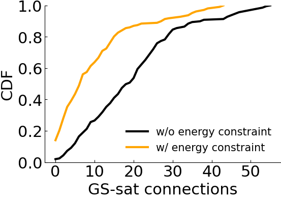
Link States. A satellite and a ground station communicate only when the satellite passes over the ground station (GS-sat connections). For GS-sat link modeling, we follow the model reported by Planet [46]. Similarly, ISLs are viable only when two satellites are close enough and have a line-of-sight (cross-sat connections). We assess the average number of active links over 5-minute windows across satellites and the distribution of link bandwidths (Figure 1-1). Our findings indicate: (a) the number of active links significantly decreases when incorporating energy constraints (energy and link constraints are dependent); (b) the median bandwidth for both GS-sat links and ISLs is around 100 Mbps, but ISLs exhibit higher variance due to the constantly changing relative positions for a pair of satellites.

(a) # of GS-sat connections.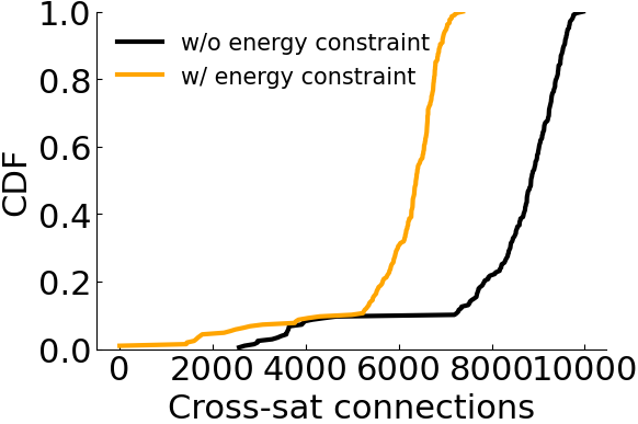

(b) # of Cross-sat connections.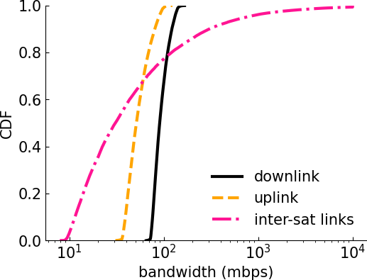

(c) Link bandwidth capacity.

Figure 1: Physical constraints (Links): The number of active communication links varies over time, constrained by bandwidths 100 Mbps.
$\blacksquare$

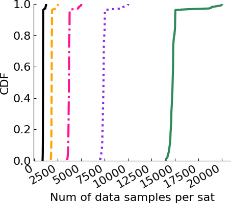
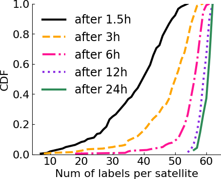
Data Availability and Heterogeneity. LEOs have limited storage capacity for imagery, and different satellites can possess significantly diverse images as they each follow a unique trajectory. For instance, a satellite recently traveled over farmland versus a dense urban area. In our study emulating a public real-world dataset, fMoW [35], we observe time-varying data availability, and the number of available labels also fluctuates over time (Figure 2-2). This high skew poses challenges for distributed training [84, 134, 62] as it biases local training, making global model convergence difficult.

Refer to caption — (a) # of available samples.

2.2 Effects of Physical Constraints on ML Training

We explore how these unique characteristics of energy, communication, and data availability constraints influence SOTA ground-based and space-based training approaches.

2.2.1 Impact on Ground-Based Training

Modern constellations depend on the BentPipe architecture [122] involving sending control commands to satellites and transmitting data back to Earth. However, downloading all high-resolution imagery to the ground is becoming increasingly difficult due to limited and intermittent bandwidth [2, 116].

To illustrate this, we model Planet’s constellation [99] along with the fMoW [35] dataset, considering energy, link, and data availability constraints (§2.1). Illustrated in Table 1, a single image captured by Planet is 300 MB [114]. We find that only 42k images, or 12.7 TB, can be downloaded to the ground per day, a figure similar to the number reported by Planet [44]. This means that if the constellation were at its full imaging capability, it would take multiple days to download the entire dataset, making it difficult for time-sensitive applications to achieve up-to-date ML models [14, 32, 87, 52]. This issue is further exacerbated for applications requiring higher-resolution images. As satellites also face onboard storage constraints (e.g., $360$ GB for FLOCK [94]), they must delete older images. We find that BentPipe struggles when it considers real-world physical constraints and has fewer images, compared to the ideal case which allows all data to be sent to the ground immediately in Table 1.

Table 1: BentPipe’s performance under varying compression performances.

Compressed Size	Ideal	100 MB	200 MB	300 MB
Downlinked Images	363,563	111,737	76,586	42,384
Percent Downloaded	100%	30.7%	21.1%	11.7%
24-hour Accuracy	59.6%	50.9%	44.1%	43.4%

2.2.2 Impact on Space-based Training

Prior works [119, 106, 31, 95] adopt federated learning for distributed ML training in space. In these approaches, each satellite, acting as a client, retrieves the ML model from the ground station and performs local ML training using its own data. The ground station, acting as the central server, receives only the model weight updates from various satellites and aggregates them to update the global ML model. This process is repeated iteratively until the global model converges. Our analysis, focusing on SOTA FL benchmarks for general resource-constrained FL, reveals that these approaches oversimplify key physical constraints of satellites and have a model accuracy degradation of 10% to 40% during ML training in space. Furthermore, while FL traditionally avoids data sharing across clients due to privacy concerns [85], ML training in space allows for data sharing among satellites within constellations, as a single company often manages them. These motivate OrbitalBrain.

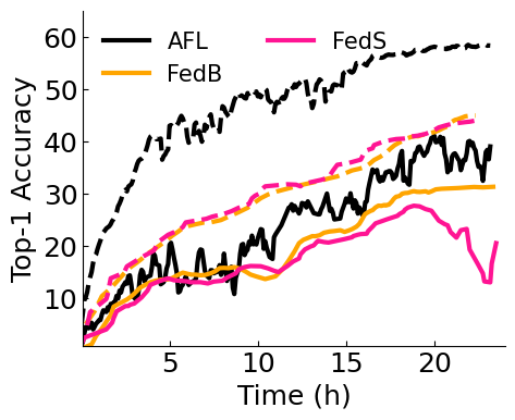
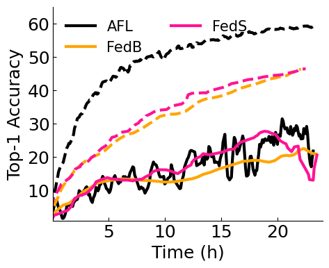
We examine the effects of these physical constraints using three SOTA benchmarks: AsyncFL (AFL) [119], FedBuff (FedB) [88], and FedSpace (FedS) [106]. We compare these methods with the fMoW dataset and two different satellite constellations (Planet [26] and Spire [27]). We consider two scenarios: one with simple constraints (i.e., GS-sat contact window determined by orbital dynamics [106, 31, 95]) and another with all constraints on energy, bandwidth, and data simultaneously (see Section 5.1 for evaluation details). All three benchmarks experience significant performance degradation when subjected to the more comprehensive practical constraints (Figure 3): the training becomes slow and unstable. This degradation is due to (i) the limited and heterogeneous local training progress resulting from energy constraints; (ii) the local model staleness caused by both link and energy constraints; and

2.2.3 Image Compression

A complementary approach to addressing the downlink bandwidth issue is to employ onboard image compression techniques. These include single-image codecs (e.g., [3, 91, 5]), neural-based autoencoders (e.g., [38, 135, 39]), and the removal of redundancies from historical observations [49]. While these methods help mitigate the problem and can be part of the solution, they only provide partial improvements. In Table 1, we analyze the result of varying compression performances, assuming that compression requires no energy (an idealistic assumption benefiting compression performance). We observe that even with a third [49] of the amount of transmitted data, only $30.7\%$ of data can be downloaded. In Figure 10(e), we evaluate integrating OrbitalBrain and BentPipe with compression techniques.

2.2.4 Satellite Predictability

Our approach, like previous satellite edge-computing research [112, 116, 106], relies on the ability to accurately forecast a satellite’s position a few ( $\sim{5}$ ) hours in advance [37, 96]. This prediction is based on Two-Line Element sets (TLEs), which provide orbital parameters and are routinely updated by official sources [26, 24]. Knowing the satellite’s position allows us to also estimate its solar power generation [100, 86, 57, 48, 108, 72, 23, 80, 115]. For our work, we assume that both the satellite’s orbital path and its power generation profile can be accurately predicted.

2.3 On-orbit labeling and training

Satellites could rely on weakly-supervised, self-supervised, or semi-supervised pipelines that produce labels (or pseudo-labels) onboard, which is a standard assumption in recent remote-sensing learning systems and space ML evaluations [7, 12, 18, 21]. Concretely, one approach is to carry compact expert (teacher) models that generate pseudo-labels for incremental adaptation of a smaller student model in orbit [82, 97]. A complementary approach is to exploit external weak supervision (e.g., geospatial priors, historical observations, or cross-sensor corroboration) and refine these labels over time, which is natural in EO where metadata and repeated coverage are abundant [36, 136, 93]. When label quality is uncertain, a practical hybrid is to triage samples: satellites downlink only low-confidence, novel, or high-utility examples for ground labeling, while the bulk of routine data is processed and used for training in orbit [43, 113, 41]. Finally, recent proposals for dedicated in-space AI infrastructure (e.g., Google’s Project Suncatcher) provide an alternative motivation for training in space while surfacing similar design constraints around optical interconnects and resource-aware scheduling [15, 55].

Summary.

We find that the physical constraints are time-varying and interdependent. These constraints present significant challenges for ground-based and distributed space-based training approaches. It is essential to thoughtfully consider these constraints when developing an effective distributed ML training solution to utilize the computational capabilities of nanosatellites in space. Fortunately, most of these resource constraints can be predicted using the satellites’ orbital dynamics and physical mechanics. This understanding informs our design approach.

3 OrbitalBrain: System Design

Problem Formulation.

Without loss of generality, we frame the problem of in-space training under physical constraints as an optimization problem formally defined in Appendix A which aims to maximize the ML convergence rate based on each satellite’s decisions regarding model aggregation (MA), data transfer (DT), and local compute (LC). However, as this optimization problem is computationally intractable due to its vast search space and the unclear relationship between different decisions and the accumulated effect on global model accuracy, we propose a new system OrbitalBrain.

System Overview.

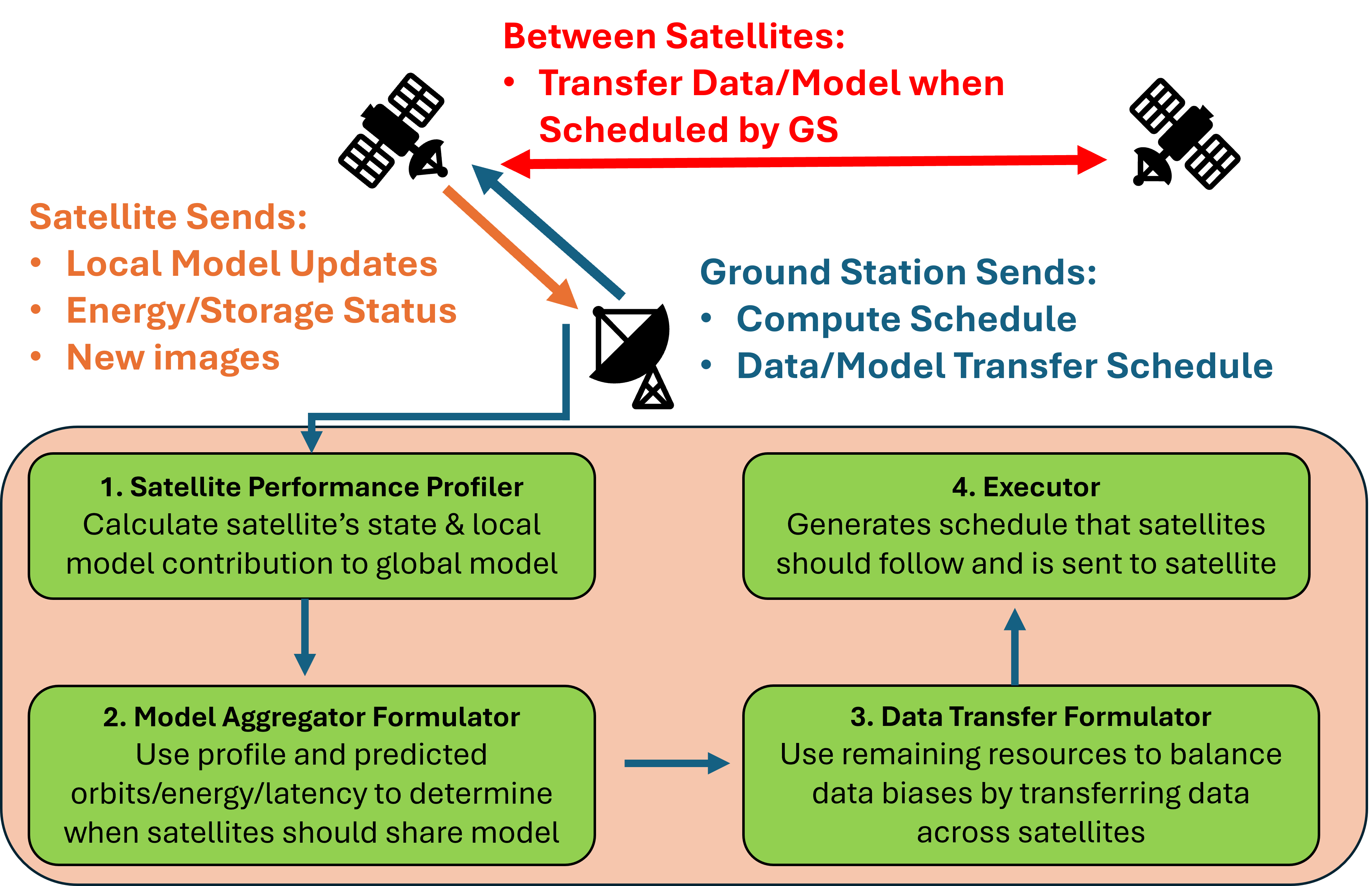
To reduce the search space for optimizing this problem, we propose a solution that disentangles the resource allocation for the computation, data transfer, and model aggregator in an approximately greedy manner. Figure 4 shows the system overview of our solution, OrbitalBrain, which consists of four main components:

1.

The performance profiler (§3.1). This component aggregates each satellite’s information at the cloud, calculating the compute utility of each satellite based on the statistics of each satellite’s local training data.
2.

The model aggregator (§3.2). The aggregator determines the feasibility and necessity of inter-sat model aggregation by considering the trade-off between aggregation gain (e.g., per-satellite model staleness, training accuracy) and execution energy/latency cost.
3.

The data transferrer (§3.3). The data transferrer considers the utility of a satellite sharing data with other satellites, which is then compared against the compute utility to determine the operation of each satellite (i.e., transfer data or local compute).
4.

The executor (§3.4). The executor will generate the effective schedule for each satellite, which is then relayed to satellites when they are in view.

This system runs on the cloud, relaying control messages to the satellite while in contact with a GS, consistent with current satellite scheduling [73]. In OrbitalBrain, we primarily utilize the cloud only as a scheduler and GS only to relay messages between satellites and the cloud.

3.1 Guided Performance Profiler

OrbitalBrain makes scheduling decisions at the cloud by creating a “profile” for each satellite. These are built by retrieving information from satellites currently connected to the ground while performing estimations based on the orbital mechanism for the rest of the satellites.

With $\mathcal{S}$ denoting the set of satellites in the constellation, for every scheduling window³³3All notations used in Section 3 can be found in Appendix C., the cloud will collect or calculate the following for each satellite $s\in\mathcal{S}$ : (1) $\eta_{s}$ , the model staleness, the number of scheduling windows since $s$ ’s last model aggregation (see §3.2). (2) $|\mathcal{D}_{s}|$ , the number of data samples the satellite used for local computation in the previous window. (3) $n^{\mathrm{comp}}_{s}$ an estimation (based on the energy trace) of the number of data samples to be computed in this window - roughly the amount of available energy divided by the time of each training iteration (4) $\mathrm{Loss}(d)$ , $s$ ’s local model training loss at the last ground connection.

This component calculates the computational utility function to determine the global model’s benefit to $s$ performing local compute.

\displaystyle\mathrm{Util}_{\mathrm{comp}}(s)

\displaystyle=n^{\mathrm{comp}}_{s}\,\sqrt{\frac{(\eta_{s}+1)^{-a}}{|\mathcal{% D}_{s}|}\sum_{d\in\mathcal{D}_{s}}\mathrm{Loss}(d)},

(1)

Intuitively, the goal of this utility function is that a local model with higher staleness (i.e. an older model) should contribute less to the global model, with some arbitrary decay factor $a>0$ (our experiments use $a=1$ ). Additionally, this function emphasizes samples that have a higher training loss ( $\frac{1}{|\mathcal{D}_{s}|}\sum_{d\in\mathcal{D}_{s}}\mathrm{Loss}(d)$ ), i.e. are less explained by the current model. This is in line with the notion of importance sampling used in ML [71, 8, 132], where a more important client is typically determined by a larger gradient norm or training loss [74]. Finally, the utility is scaled by $n^{\mathrm{comp}}_{s}$ since there is more value if we anticipate that this satellite will perform more computation in future rounds.

3.2 Model Aggregation (MA) across Satellites

OrbitalBrain determines the feasibility of aggregating all satellite’s profiled models with other satellites over ISLs (aggregation is the process of combining locally trained models into a single global model by averaging each client’s model weights).

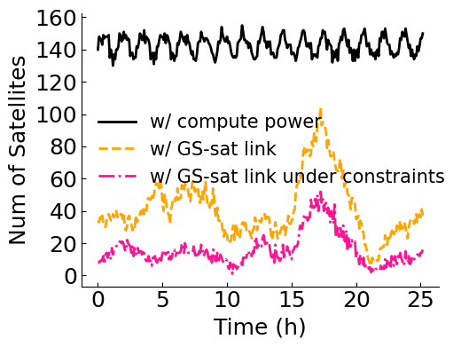
By communicating through ISLs, this mechanism enables more continual aggregation than only utilizing ground station (GS) connections. This can be seen in Figure 5 where the GS-sat connections of Planet’s constellation for a whole day are shown. As time evolves, the number of satellites in view of the ground (orange) fluctuates between 10 at 21h and 100 at 18h. Unfortunately, only approximately $1/3$ of these satellites (pink) can actually establish these GS-sat connections if we incorporate energy constraints (§2.1). Accordingly, most satellites which have sufficient compute power (black), have no ability to gather new model updates. This leads to a satellite spending energy to produce a stale, old model update.

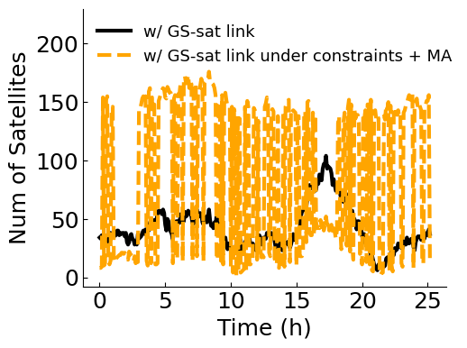
The advantage of OrbitalBrain’s MA mechanism is shown in Figure 5 where from $4$ h- $15$ h and from $19$ h- $25$ h OrbitalBrain has almost $4\times$ more local updates when MA is enabled.

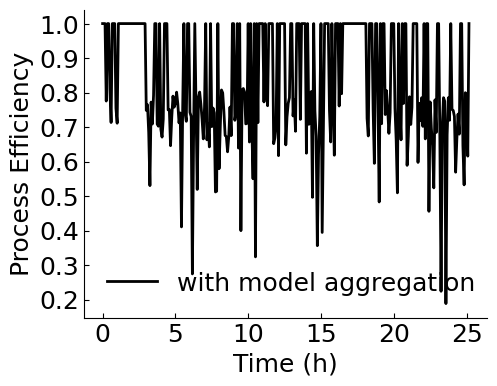
However, MA induces extra time and energy costs, reducing the computation efficiency (the ratio of energy for computing relative to a satellite’s available energy) as shown in Figure 5. For example, at $24$ h, only $20\%$ of data samples can be processed because most energy is used for inter-satellite MA.

To determine if MA is valuable in a given scheduling window, OrbitalBrain follows a threshold-based process, comparing the MA-enabled rewards with the cost in energy and time (we also ensure that MA can complete in a given scheduling window). This component utilizes the predictable orbit and energy (§2.2.4) to find (1) $\mathcal{S}_{c}$ , the set of satellites which in this scheduling window have sufficient compute power, and (2) $\mathcal{S}_{cc}$ , a subset of $\mathcal{S}_{c}$ only including the satellites with communication ability to the ground. Note that $\mathcal{S}_{c}\setminus\mathcal{S}_{cc}$ is the set containing satellites with sufficient energy but no GS-sat connections. Additionally, this calculation utilizes each satellite’s model’s staleness, $\eta_{s}$ (§3.1), the current number of scheduling windows since this satellite’s model was aggregated with the global model (will be reset to 0 if MA occurs).

We determine if it is valuable to perform MA by testing:

	$\displaystyle\frac{\mathrm{Util}(\mathcal{S}_{c}\setminus\mathcal{S}_{cc},% \boldsymbol{\epsilon})}{\mathrm{Util}(\mathcal{S}_{cc},\mathbf{1})}>\theta_{0}% (t+1)^{-b},$			(2)
	$\displaystyle\text{where}\nobreak\ \nobreak\ \mathrm{Util}(\mathcal{S},% \boldsymbol{\epsilon})$	$\displaystyle\!=\!\left(\frac{\sum_{s\in\mathcal{S}}\eta_{s}}{\|\mathcal{S}\|}+1% \right)^{-a}\!\!\sum_{s\in\mathcal{S}}\epsilon_{s}\mathrm{Util}_{\mathrm{comp}% }(s).$

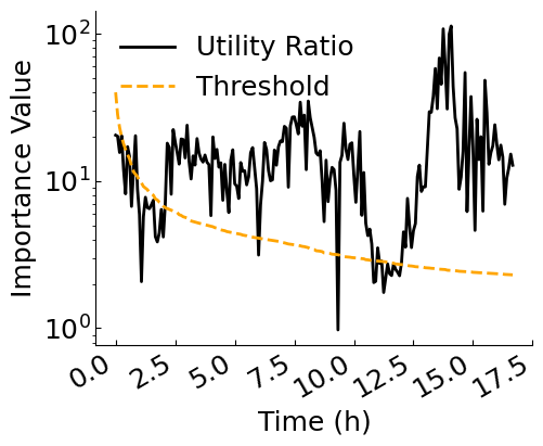
The insight behind Eq 2 is that the utility of model aggregation, $Util(\mathcal{S}_{c}\setminus\mathcal{S}_{cc},\epsilon)$ , should be larger than these satellite spending their energy on local compute $Util(\mathcal{S}_{c},1)$ . For MA to be beneficial, the ratio between these utilities should be larger than the term $\theta_{0}(t+1)^{-b}$ where $\theta_{0}$ is an initial threshold and $b$ is a time-based decay factor. This threshold ensures that at early epochs, satellites train their local model. As these models become more developed, MA will be prioritized.

This threshold’s time-varying nature responds to the empirical observation that the value of MA is larger at later stages of the training process. Figure 5 illustrates the utility ratio in Eq (2) and the time-varying threshold based on Planet’s constellations.

Additionally, if MA is scheduled, OrbitalBrain determines which satellites should communicate by finding the shortest-path tree for $\mathcal{S}_{c}$ where the root is the satellite with the most ISLs. Finding this tree is an $O(|I|\log(|S|))$ operation where $|I|$ is the number of ISLs $(|I|<|S|^{2})$ and $|S|$ is the number of satellites.

3.3 Enabling Data Transfer (DT)

One problem that emerges from a satellite’s fixed orbit is that each satellite will not contain all labels evenly. This causes local training to overfit to a satellite’s own label distribution [84, 134, 62]. Most traditional FL approaches only rely on model aggregation to alleviate this inbalance by averaging each device’s biased model weights [105, 88, 78]. This is primarily motivated by the privacy settings that FL adheres to. However, we observe that since all satellites in this framework are controlled by one company (i.e. Planet or Spire), directly transferring data between satellites is permitted. This allows for direct averaging of labels instead of expending energy training an unbalanced model which must later be averaged.

Our data transfer component first (1) calculates each satellite’s data utility, that is how useful each satellite is to achieving balanced labels. (2) the usefulness of sharing data between two satellites, and (3) determines between multiple satellites in view, which links should be utilized.

The cloud scheduler retrieves the data distribution of each satellite when a satellite connects with a ground station. It continues to keep track of the expected change in each satellite’s distribution when DT is scheduled, correcting this estimation when a GS-sat connection occurs.

Intuitively, a satellite $s$ has a larger data utility if it has more balanced data and sufficient energy for local computation:

\displaystyle\mathrm{Util}_{\mathrm{data}}(s)=n^{\mathrm{collect}}_{s}(1-F_{% \mathrm{dis}}(\mathbf{\ell}_{s}))^{n^{\mathrm{comp}}_{s}}

(3)

where $F_{\mathrm{dis}}(\mathbf{\ell}_{s})$ indicates the Jensen–Shannon divergence (JSD), a measure of the label distances between a satellite’s current label distribution $\mathbf{\ell}_{s}$ and the i.i.d (perfectly balanced) label distribution. $n^{\mathrm{collect}}_{s}$ and $n^{\mathrm{comp}}_{s}$ are the numbers of data samples to be collected and computed under energy constraints (§3.1).

The transfer utility for transferring data between two satellites depends on both the transmitting and receiving satellite’s current label distribution, formulated as:

\displaystyle\mathrm{Util}_{\mathrm{tr}}(s,s^{\prime})=F_{\mathrm{dis}}(% \mathbf{\ell}_{s^{\prime}})-F_{\mathrm{dis}}(n^{t}_{ss^{\prime}}\,\frac{% \mathbf{\ell}_{s}}{|\mathbf{\ell}_{s}|}+\mathbf{\ell}_{s^{\prime}}),

(4)

where $n^{t}_{ss^{\prime}}$ indicates an estimation of the number of Transferred data samples from $s$ to $s^{\prime}$ if transfer was to happen-energy and storage permitting. The transfer utility is large if after receiving the samples from $s$ , $s^{\prime}$ will have a smaller distance to the ideal i.i.d. data distribution.

Finally, based on the data and transfer utilities, we compute the link utility for each possible pair of satellites in view of each other, determining whether a selected link (a pair of satellites) is the best possible, additionally ensuring that transferring data is more beneficial than a satellite training on its own current data.

OrbitalBrain selects the link $(s,s^{\prime})$ with the largest utility iteratively for data transfer ( $s\neq s^{\prime}$ ) or local computation ( $s=s^{\prime}$ ) and terminates when all remaining link utilities are negative. A negative $\mathrm{Util}_{\mathrm{tr}}(s,s^{\prime})$ means that data transfer cannot make the data distribution of the destination closer to being i.i.d.

\mathrm{Util}_{\mathrm{link}}(s,s^{\prime})=\begin{cases}\mathrm{Util}_{% \mathrm{tr}}(s,s^{\prime})\,\mathrm{Util}^{*}_{\mathrm{data}}(s^{\prime})&% \text{if $s\neq s^{\prime}$}\\ \xi\,\mathrm{Util}_{\mathrm{data}}(s^{\prime})&\text{if $s=s^{\prime}$}\end{cases}

(5)

where $\mathrm{Util}^{*}_{\mathrm{data}}(s^{\prime})$ represents the data utility of satellite $s^{\prime}$ after receiving the data samples from $s$ . $\xi$ is a self-computation utility parameter that determines how much to emphasize local training vs transferring.

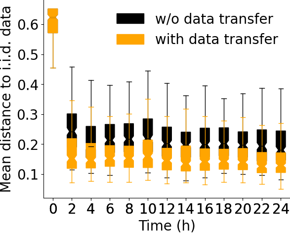
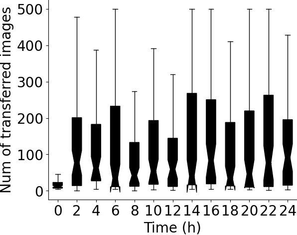
Figure 6 verifies the effectiveness of OrbitalBrain’s data transfer strategy. With data transfer, the distance to the i.i.d. data distribution (uniform label distribution) for each of the Planet constellations decreases significantly over time, with a lower median value (from $0.21$ to $0.12$ ) in Figure 6. Figure 6 shows the number of transferred images across those satellites at each scheduling window, spanning from $20$ to $500$ , which is determined by the bandwidth of ISLs and the energy constraints.

Algorithm 1 OrbitalBrain’s ML training framework (runs on the ground station).

3.4 Executor: Putting It All Together

We put all components together in Algorithm 1. The total runtime is $\mathcal{O}(S^{2}log(S))$ where $S$ is the number of satellites. In each scheduling window $t$ of length $T_{t}$ , the performance profiler first retrieves the satellite information for profiling, including the training loss, staleness $H$ , energy trace $E$ , on-board storage $M$ , label distribution $\mathbf{\ell}$ , and the link topology $G$ (line 2 - $\mathcal{O}(S)$ ). It updates the compute utility based on Eq. (1) (line 3 - $\mathcal{O}(S)$ ) and detects each satellite’s status under the energy constraints (line 4 - $\mathcal{O}(S)$ ). Given the ISL connectivity topology $G_{ISL}$ , OrbitalBrain checks the MA feasibility and resulting compute efficiency (line 5 - $\mathcal{O}(S^{2}log(S))$ ). If deemed beneficial, it schedules the local training and MA sequentially for those energy-sufficient satellites $\mathcal{S}_{c}$ , deriving the local model updates $\mathcal{P}$ (lines 6-8 - $\mathcal{O}(S)$ ). The empty second argument in ExecuteTraining in line 8 indicates the absence of data transfer. Otherwise, it allocates compute/communication resources for data transfer based on the computed link utility iteratively (lines 9-15 - $\mathcal{O}(S^{2})$ ). It then schedules the local computation and data transfer for different satellites (line 16 - $\mathcal{O}(S)$ ). Finally, it schedules when local model updates and training statistics (implicit in $\mathcal{P}$ ) are sent to the ground to update the global model (line 17 - $\mathcal{O}(S)$ ). Once this schedule is created on in the cloud, it will be uploaded to a satellite when each satellite comes into contact with a ground station.

4 Implementation

We implement OrbitalBrain in Python ( $3,556$ lines) for orbital simulation and distributed ML training in space. OrbitalBrain’s orbital simulation based on CosmicBeats [101] outputs the energy traces, link topology, and data streamed for each satellite as the number of data samples manipulated for different purposes, such as the images collected, transferred, and computed at each scheduling window. Our ML simulator built on top of a federated learning framework (FLUTE [47]) takes these traces to update the satellite profiles/link utility for inter-sat communication and simulate distributed ML training in space under physical constraints. OrbitalBrain can be easily incorporated with other FL frameworks such as FjORD [61] and FedSEA [110]. We use OpenMPI [53] as the backbone for multi-worker distributed ML training.

To make our simulator faithful to the real world, we build our orbital emulation on CosmicBeats, which provides verified models for orbit propagation, contact opportunities, power dynamics, and data/storage state; this framework has been validated against an actual nanosatellite launch [104, 101, 100, 103, 30]. These models naturally yield scheduled ground-station (GS)-to-satellite and cross-satellite connectivity graphs (we use 5-minute granularity [104]). We assume that satellite positions (and thus line-of-sight (LOS) opportunities) are predictable ahead from Two-Line Elements (TLEs), consistent with empirical accuracy studies of NORAD/TLE-based propagation [37, 96, 116] and standard premises in satellite-network scheduling [114, 106]. For GS-sat links, we parameterize bandwidth and energy costs using reported Planet radio characteristics and measurements [45]. For Inter-Satellite Links (ISLs), we model feasibility via range/LOS constraints and bounded link rates (100 Mbps). Overall, we believe these assumptions align with our target scenarios, and the primary uncertainty for our simulator’s realism lies in how scarce energy and bandwidth are allocated across local compute and data transfer under predictable orbital constraints [59, 65, 129, 124, 42, 41, 113, 114, 89].

5 Evaluation

We evaluate OrbitalBrain’s performance with two satellite constellations on two space tasks. The key results are:

$\blacksquare$

Overall Performance. OrbitalBrain outperforms SOTA baselines for various space tasks. It achieves $1.52\times$ - $12.4\times$ speedup in time-to-accuracy with $1.9\%$ - $49.5\%$ final model accuracy improvement.
$\blacksquare$

Ablation Study. OrbitalBrain optimizes the non-i.i.d data distribution and model staleness effectively with data transfer and modal aggregation under physical constraints.
$\blacksquare$

Robustness & Sensitivity. OrbitalBrain consistently performs well in various scenarios, such as varying cloudy images, image compression & resolution, and participating satellites. We also show effective collaborative learning by incorporating GS and satellites for ML in space.
$\blacksquare$

Approaching the Ideal Case. OrbitalBrain narrows the performance gap in comparison to its ideal counterparts.

5.1 Methodology

Constellations, Tasks, Dataset. For the orbital emulation, we utilize 24-hour TLE traces of Planet [26] (with 207 satellites) and Spire [27] (with 117 satellites). We employ the locations of Planet’s 12 global ground stations [114]. We assess OrbitalBrain on two space tasks.

$\blacksquare$

Functional Map of the World (fMoW) [35] provides $360k$ RGB images captured by Digital Constellations [90] in 363 UTM zones across the globe. We use DenseNet [63] and calculate the top-1 accuracy for land function prediction among $62$ categories.
$\blacksquare$

So2Sat [137] collects 400k multi-spectral images from Sentinel-2 multi-spectral instrument (MSI) [4], covering $43$ cities. We use ResNet [60] and calculate the top-1 accuracy for 17-category climate zone classification.

We only train the final five layers of DenseNet-161 [63] (~23M parameters) and ResNet-50 [60] (~16M parameters), which is comparable to ResNet-18 (~11M parameters). With the Jetson Orin Nano 4 GB GPU [50], we achieve satisfactory inference speeds, with DenseNet-161 operating at 401 frames per second (FPS) and ResNet-50 at 621 FPS. These speeds are well-suited for the usual satellite imaging rates of 0.3 FPS.

To emulate the data streaming process for each satellite as it orbits the Earth, we assign each data sample to its associated geo-locations and rank them by their collection time for the same location. Each satellite collects several data samples under its energy constraints while orbiting the Earth in each window. Similar to the vast majority of FL work [69], we assume the satellite generates labeled data for ML training using unsupervised or semi-supervised techniques [6, 22, 13, 19].

Baselines and Metrics.

We implement and compare five baselines with OrbitalBrain under satellites’ physical constraints, including the centralized training (i.e., BentPipe (BP) [122]) and four FL approaches (i.e., AsyncFL (AFL) [119], SyncFL (SFL) [20], FedBuff (FedB) [88], and FedSpace (FedS) [106]). In SyncFL [20], the GS waits for the local gradients from a certain number of non-straggler satellites ( $50\%$ ) before updating and distributing its global model. In contrast, GS in AsyncFL updates the global model at its best efforts whenever local gradients are available from satellites. FedBuff balances the SyncFL and AsyncFL by buffering the local gradients from satellites and updating the global model only when its size reaches a threshold $B$ (default 32). The SOTA ML framework in space, FedSpace, dynamically schedules model aggregation based on the deterministic connectivity and its performance estimation from model staleness.

Our primary performance metric is time-to-accuracy [74, 76], which comprises the final test accuracy of the global ML model and its training wall clock time. Specifically, we calculate the final model accuracy by averaging the test accuracy over the last five scheduling windows. We measure OrbitalBrain’s wall clock time required to achieve the final test accuracy of the baselines, enabling us to determine its speedups over them (Table 3).

Parameter Setting.

We set the orbital sampling period $T_{t}$ (scheduling window) as $5$ mins. Each satellite has an onboard storage of $360$ GB [94] to store the imagery data with the size of $200$ MB and $400$ MB for fMoW [35] and So2Sat [137]. Once reaching $90\%$ of its storage, the satellite will delete $50\%$ of the oldest data samples. We tune the hyperparameters of ML training for different tasks, which yields minibatch sizes at $24$ and $64$ for fMoW and So2Sat, with the learning rate of $5e$ - $3$ and $1e$ - $3$ , respectively. We empirically determine OrbitalBrain’s parameters throughout the evaluation, where the staleness decay factor $a$ is $1$ (Eq 1). The initial process efficiency $\epsilon$ is $0.9$ as setting up an ISL takes over 10 seconds [59] (Eq 2). We have the initial threshold $\theta_{0}=40$ and decay factor $b=0.5$ for the threshold-determined model aggregation (line 5 in Algorithm 1). The self-computation utility is set at $20$ for inter-satellite data transfer (Eq 5).

5.2 End-to-End Performance

Table 2: OrbitalBrain improves the final test accuracy after 24 hours over all five baselines, under various space tasks, ML models, and satellite constellations.

Space Tasks	Dataset	Model	Const.	BP	SFL	AFL	FedB	FedS	OrbitalBrain
Land Function	fMoW (62 classes) [35]	DenseNet	Planet	47.3%	3.3%	37.4%	17.8%	31.2%	52.8%
Recognition	fMoW (62 classes) [35]	DenseNet	Spire	50.2%	5.6%	24.2%	14.7%	18.0%	59.2%
Climate Zone	So2Sat (17 classes)[137]	ResNet	Planet	46.0%	10.5%	17.8%	14.8%	10.5%	47.9%
Recognition	So2Sat (17 classes)[137]	ResNet	Spire	43.0%	9.4%	35.1%	20.6%	19.2%	47.1%

Table 2 and 3 summarize OrbitalBrain’s improvements in final test accuracy and speedups with less wall clock time.

OrbitalBrain improves the final test accuracy with more i.i.d data.

For the most difficult task, fMoW, OrbitalBrain achieves much higher final test accuracy of $52.8\%$ and $59.2\%$ over existing baselines, with the improvement of $5.5\%$ - $49.5\%$ on Planet and Spire. Figure 7 and 7 show the time-to-accuracy curve for fMoW. fMoW’s high non-i.i.d data renders a fluctuating trend for most baselines except the steady but slow SyncFL and BentPipe. In contrast, OrbitalBrain allocates some satellites for inter-satellite data transfer instead of the local computation to make data distribution more balanced for each satellite, resulting in a more steady training process with higher final test accuracy.

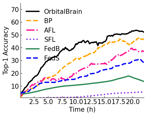
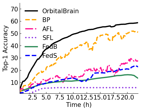
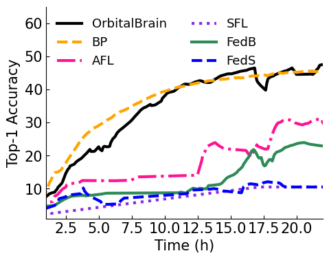
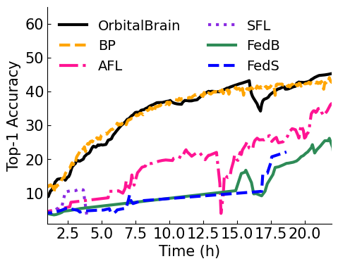
Figure 7 and 7 shows that OrbitalBrain achieves similar steady training trends with much higher test accuracy than the distributed ML baselines on the So2Sat dataset, under Planet and Spire constellations. Compared to fMoW, So2Sat only has 17 labels for the climate zone recognition, which favors BentPipe to train a good model even with much fewer data samples collected in the ground stations. Therefore, OrbitalBrain only improves BentPipe slightly, with a higher accuracy of $1.9\%$ and $4.1\%$ for climate zone recognition. We attribute this to our inter-satellite model aggregation to reduce model staleness. With only a few satellites connecting to the ground per window, satellites with a stale global model degrade aggregation quality when downloading their local models to the ground. OrbitalBrain sacrifices certain compute resources for inter-satellite communication to improve the quality of global model aggregation with fewer stale model updates.

Table 3: OrbitalBrain’s speedup of time consumption to reach the same final accuracy as baselines.

Dataset	Constellation	BP	AFL	FedS
fMoW	Planet	1.55 $\times$	3.25 $\times$	4.33 $\times$
fMoW	Spire	1.52 $\times$	8.73 $\times$	9.58 $\times$
So2Sat	Planet	2.22 $\times$	8.65 $\times$	12.42 $\times$
So2Sat	Spire	1.61 $\times$	3.21 $\times$	9.24 $\times$

OrbitalBrain speeds up the global model training by enabling frequent model aggregation across satellites.

Table 3 presents the time it takes for OrbitalBrain’s to reach each baseline’s final test accuracy after a $24$ -hr ML training. We make two observations. First, OrbitalBrain achieves a robust speedup across various ML models, image types, and constellations. For these two ML tasks, OrbitalBrain achieves higher speedup for fMoW and So2Sat because these two datasets were captured from the Earth with greater diversity, which leads to more difficult non-i.i.d. data issues for the baselines. Second, OrbitalBrain only needs several rounds of training warm-up and its efficiency increases over time. OrbitalBrain fully exploits the computation resources of all satellites with sufficient energy even if they cannot communicate to the ground. Such an edge computing framework makes it start faster than the centralized BentPipe [122], especially for the diverse fMoW dataset with much more data labels.

5.3 Component-wise Analysis

To assess the effectiveness of OrbitalBrain’s key components, we evaluate two breakdown versions of the system.

OrbitalBrain ensures the most up-to-date global model through inter-satellite model aggregation.

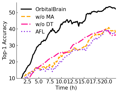
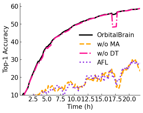
The omission of inter-satellite model aggregation (MA) leads to a notable decrease in performance, as indicated by Table 4, which shows a reduction of $14.7\%$ and $36.1\%$ in the final test accuracy for the fMoW dataset. The time required for the breakdown versions to achieve the same test accuracy is $2.5\times$ to $8.5\times$ longer. Figure 8 compares the performance of OrbitalBrain without inter-satellite MA (orange) to that of AsyncFL (purple). Although OrbitalBrain without inter-satellite MA still slightly outperforms AsyncFL, it does not reach the full potential exhibited by the complete OrbitalBrain (black). An exception is the fMoW dataset with the Spire constellation, where the performance of OrbitalBrain without MA converges with that of AsyncFL. This can be attributed to the geographically widespread Spire constellation, which results in a reduced number and bandwidth of inter-satellite links. Consequently, there is a significant decrease in the volume of images transferred between satellites, leading to similar performance for both approaches.

Table 4: OrbitalBrain’s ablation study indicates the final test accuracy decrement and training slowdown.

Constell.	w/o Model Aggreg.		w/o Data Transfer
Constell.	Acc	Slowdown	Acc	Slowdown
Planet	14.7% $\downarrow$	2.5 $\times$	11.3% $\downarrow$	2.2 $\times$
Spire	36.1% $\downarrow$	8.5 $\times$	0.3% $\downarrow$	1.0

OrbitalBrain optimizes each satellite’s data distribution by selectively substituting local computation with data transfer.

OrbitalBrain without DT (data transfer) experiences a noticeable performance reduction. Table 4 shows that the degradation can reach up to $11.3\%$ in final accuracy and $2.2\times$ in time-to-accuracy for OrbitalBrain without DT on the Planet constellation. In the Spire constellation [27], OrbitalBrain without DT matches AsyncFL’s training trend, as the well-distributed satellites collect balanced data, effectively training a global model through model aggregation alone without DT.

OrbitalBrain reduces model staleness and utilizes compute resources.

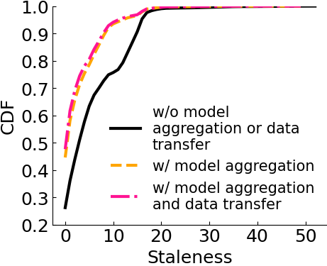
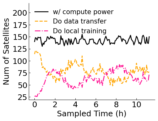
In Figure 9, we analyze the effectiveness of our MA and DT strategy utilizing fMoW and Planet. In Figure 9, we plot a CDF of each satellite’s model staleness at every scheduling window. Model staleness is the number of scheduling windows since a satellite’s local model was aggregated with the global model. We observe in $90\%$ of the scheduling windows, each satellite’s staleness was smaller than $8$ scheduling windows (from $18$ ). In Figure 9, we analyze when OrbitalBrain utilizes the DT process, observing that more satellites transfer data at the beginning when the data distribution is more unbalanced. OrbitalBrain continues to assign DT and local computing dynamically depending on how the distribution evolves, fully exploiting available energy resources.

5.4 Robustness and Sensitivity

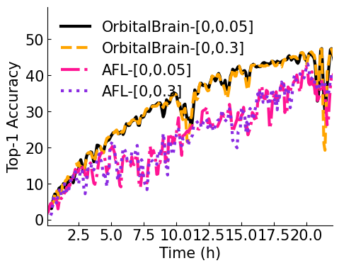
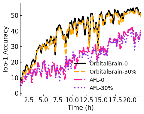
We demonstrate OrbitalBrain’s robustness across four distinct scenarios: 1) What is the impact on space training when integrating both satellites and ground-based datacenter training? 2) How does the number of participating satellites affect OrbitalBrain’s strategies for distributed training in space? 3) Is OrbitalBrain resilient to cloudy images collected by LEO nanosatellites? 4) How does OrbitalBrain perform when dealing with various compression image sizes and varying resolutions from heterogeneous sensors on nanosatellites? We use fMoW [35]+Planet [26] in this study.

Collaboration between satellites and ground stations/datacenters.

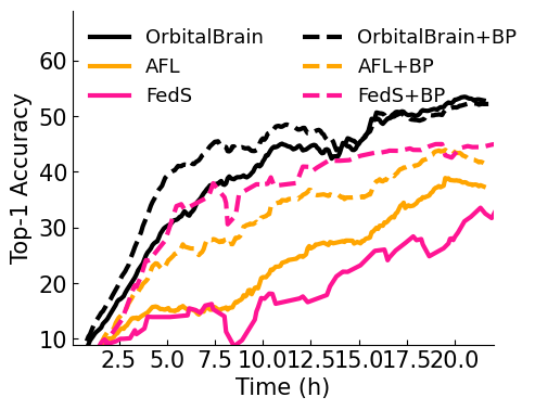
Although OrbitalBrain is primarily designed for orbital edge computing, it also facilitates collaborative training between satellites and traditional ground-based compute (either at a ground station or in a cloud/datacenter). By combining model updates received from satellites with the ground-based model using BentPipe (represented by dashed lines), Figure 10(a) shows that both OrbitalBrain and FedSpace achieve a more stable training progression and higher final accuracy for both satellite constellations. AsyncFL also reaches a higher final accuracy, albeit with a more volatile trend, owing to the frequent integration of outdated models from the satellites. In addition, OrbitalBrain ensures consistency between the ML model trained in orbit and the one trained on the ground, thereby outperforming the other two baseline methods even when including collaboration with BentPipe.

Impact of participating satellites.

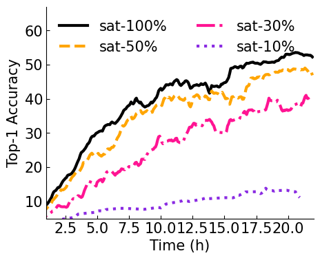
We vary the participation ratio in the constellation. Figure 10(b) shows OrbitalBrain’s performance on Planet and Spire. As we see, OrbitalBrain suffers significantly when only $30\%$ satellites join the ML training. The reasons for this are twofold. First, with fewer participating satellites, there are fewer model updates sent to the ground station, which impedes the utilization of the imagery data collected by the satellites. Second, a reduced number of satellites necessitates more orbital cycles to gather data samples, thus decelerating the collaborative training efficiency of OrbitalBrain for a global DNN model. OrbitalBrain demonstrates improved performance with higher numbers of participating satellites. A participation rate of over $50\%$ ensures satisfactory performance.

Impact of Cloudy images.

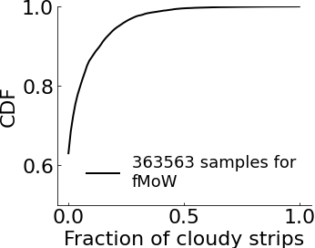
A unique challenge for Earth observation is that some image patches are obscured by seasonal snow or clouds [109]. Such image data must be either filtered out or specifically processed for ML training. Figure 10(c) initially presents the proportion of the fMoW dataset’s [35] image strips that are completely obscured by clouds, on a scale from $0$ to $1$ (only $40\%$ of these images are affected by any cloud cover). We filter the fMoW images using different cloud cover thresholds (i.e., $0.05$ and $0.3$ ), which results in $80\%$ and $97\%$ of the total images being retained, respectively. Figure 10(d) depicts the training performance of OrbitalBrain and AsyncFL. It is observed that AsyncFL’s performance becomes more erratic with an increase in cloudy images (e.g., hours $10$ and $23$ for the purple curve). In contrast, OrbitalBrain maintains consistent performance with a stable training trend over time by facilitating inter-satellite data transfer. This data-sharing strategy helps mitigate the adverse effects of excessive cloudy images on local model training.

Impact of compression performance.

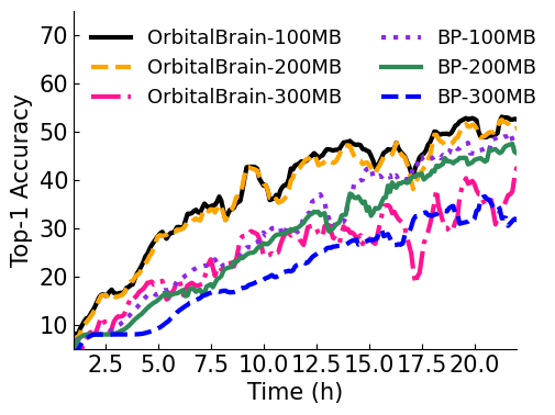
We evaluate the impact of a compressed image size of $100$ MB, $200$ MB, and $300$ MB. We assume that compression requires no energy despite multiple compression works [40] utilizing GPUs. Figure 10(e) shows a larger image slows down the data downloading and transfer efficiency, resulting in training degradation. We observe that both OrbitalBrain and BentPipe perform better as the compression performance increases. We observe that OrbitalBrain with 100MB and 200MB outperforms all BentPipe approaches. Additionally, we observe that OrbitalBrain at 300MB outperforms BentPipe at the same compression ratio, almost achieving the same performance as BentPipe 200MB.

Impact of Varying Resolutions.

We also examine OrbitalBrain and AsyncFL for imagery data with various resolutions. fMoW [35] provides $360k$ images with a median ground sample distance (GSD) of $0.5m$ [35]. To evaluate the impact of image resolutions, we randomly select a certain number of satellites (e.g., $30\%$ ) and rescale their imagery data to a $4\times$ larger resolution. Figure 10(f) demonstrates the time-to-accuracy performance, which verifies the necessity of data transfer for a steady training trend. With images of different resolutions, AsyncFL suffers significantly (e.g., 15-20 hours for the pink and purple) while OrbitalBrain is resilient with overlapping training trends.

5.5 Comparison with the Ideal Cases

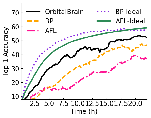
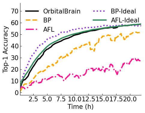
In this section, we propose two ideal baseline scenarios to showcase the effectiveness of OrbitalBrain: (1) BentPipe-ideal assumes that each satellite observes i.i.d. data and downlinks all collected samples to the ground with no link-capacity constraints. We assume this baseline expends the same total energy as our full satellite constellation if it was to train a global model on 10,000 samples. (2) AsyncFL-ideal also assigns i.i.d data to each satellite using random data assignment. Each satellite consistently communicates with the ground for global model distribution and aggregation.

We draw three conclusions from Figure 11: (1) Both BentPipe and AsyncFL experience significant difficulties due to their non-i.i.d data and intermittent connections with the ground for model aggregation, resulting in a substantial performance gap compared to their ideal scenarios. (2) A centralized training method with sufficient data, such as BentPipe-ideal, achieves the best performance (purple). However, it performs poorly when limited to non-i.i.d data samples under link constraints (orange). (3) By facilitating inter-satellite model aggregation and data transfer, OrbitalBrain optimizes data distribution and model staleness for each satellite, bringing it closer to the AsyncFL-ideal.

6 Related Work

Resource-Constrained Federated Learning.

A growing body of research in FL focuses on its application in resource-constrained environments, such as the Internet of Things (IoT), robots, and drones [119, 64]. Existing work typically targets a specific limited resource (e.g., computation, memory, and energy) and proposes solutions to improve the efficiency of that particular resource. For example, pruned or quantized models have been utilized to reduce computation and communication overheads [67, 61, 75, 9]. Our work is largely complementary to these approaches, as we examine the trade-offs of various operational decisions to optimize the use of limited resources in a previously unexplored context.

Compared to conventional FL in mobile networks, the new scale of both the time and the region traversed are much larger in the nanosatellite context. This is unlike prior works in areas such as drones or mobile phones because these nanosatellites are subjected to their orbital paths. Drones, however, are often remotely controlled and can move in new directions [64]. This subjected orbital path presents a great opportunity for research as our system leverages this property extensively (§2.2.4). Additionally, satellites have more prolonged communication gaps (order of hours) while facing substantial transmission delays due to the long distances involved (often requiring pre-computation of scheduling)[83].

Model Aggregation in Federated Learning.

A large body of work studies different aspects of FL [84, 69]. FL model aggregation can be broadly classified into Synchronous FL (SyncFL) [20] and Asynchronous FL (AsyncFL) [88]. SyncFL ensures the convergence of the global model [84, 77] by waiting for slower clients [69, 131], but this approach inevitably results in increased latency. In contrast, AsyncFL [119, 125, 126] avoids stragglers to improve time efficiency but must consider convergence analysis [34, 33] and model staleness for biased aggregation [107, 29]. Our solution also takes into account the trade-offs between stragglers and model staleness. Additionally, our system is more comprehensive, considering data sharing, local training, and adherence to interdependent physical constraints – all designed for the nanosatellite context.

Federated Learning in Space.

FL has been investigated for use in space-based training [31, 95, 106], where each satellite only sends its local model updates to the ground, avoiding the need to download high-resolution data. However, these studies either adopt simplistic orbital assumptions or overlook certain constraints. For instance, FedSpace [106] only considers satellite-to-ground station connectivity for communication, neglecting energy, storage, or data streaming constraints. In contrast, we use real satellite traces to design a system adhering to the physical constraints of satellites, asserting that multiple models of ours (energy, link, storage) match reported data from actual satellite launches [46, 101, 94]. We utilize this data to develop a first-of-its-kind ML training simulator using these traces, conducting extensive comparisons with existing solutions in our evaluation. Our approach also differs from FL, as we do not require data isolation for privacy concerns among satellites [105, 88, 78]. Consequently, OrbitalBrain thoroughly leverages inter-satellite data transfer and model aggregation for efficient ML training in space.

Orbital Edge Computing for Satellites.

The concept of orbital edge computing [42, 40, 112, 114] involves equipping satellites with computing devices to derive insights in space, which has been implemented in multiple real satellite missions [54, 121]. These satellites are often equipped with new advancements in radiation shielding [120] and error-correcting codes [117]. Additionally existing inference pipelines [42, 112] focus on running image filtering or ML inference on satellites, while our work targets more complex training tasks to keep these edge models up-to-date.

7 Conclusion

Training ML models in space offers a promising alternative to conventional training, especially in the era of rapidly growing LEO nanosatellites. We develop a simulator for distributed ML training in space, demonstrating the physical constraints of satellites pose significant challenges. We introduce OrbitalBrain, a framework that balances trade-offs among data transfer, model aggregation, and local training. OrbitalBrain estimates the utility of various operations using predictable physical constraints and local training statistics. Evaluations across two space ML tasks and two satellite constellations reveal OrbitalBrain achieves a $1.52\times$ - $12.4\times$ speed-up in time-to-accuracy while always achieving a higher final model accuracy over existing centralized and federated learning baselines. We hope our findings, simulator, and datasets encourage further research to address this emerging problem.

References

[1] Spire global nanosatellite constellation. https://www.eoportal.org/satellite-missions/spire-global, 2017.
[2] Planetscope - Dove Satellite Constellation (3m). https://www.satimagingcorp.com/satellite-sensors/other-satellite-sensors/dove-3m/, 2021.
[3] Masud Ibn Afjal, Md. Al Mamun, and Md. Palash Uddin. Band reordering heuristics for lossless satellite image compression with 3d-calic and CCSDS. J. Vis. Commun. Image Represent., 59:514–526, 2019. doi:10.1016/J.JVCIR.2019.01.042.
[4] European Space Agency. Sentinel-2 msi user guide. In https://sentinel.esa.int/web/sentinel/user-guides/sentinel-2-msi, Retrieved in 2022.
[5] Bruno Aiazzi, Luciano Alparone, Stefano Baronti, and Cinzia Lastri. Crisp and fuzzy adaptive spectral predictions for lossless and near-lossless compression of hyperspectral imagery. IEEE Geosci. Remote. Sens. Lett., 4(4):532–536, 2007. doi:10.1109/LGRS.2007.900695.
[6] Peri Akiva, Matthew Purri, Kristin Dana, Beth Tellman, and Tyler Anderson. H2o-net: Self-supervised flood segmentation via adversarial domain adaptation and label refinement. In Proceedings of the IEEE/CVF Winter Conference on Applications of Computer Vision, pages 111–122, 2021. doi:10.1109/WACV48630.2021.00016.
[7] Peri Akiva, Matthew Purri, Kristin Dana, Kristin Tellman, and Tyler Anderson. H2o-net: Self-supervised flood segmentation via adversarial domain adaptation and label refinement. In Proceedings of the IEEE/CVF Winter Conference on Applications of Computer Vision (WACV), 2021.
[8] Guillaume Alain, Alex Lamb, Chinnadhurai Sankar, Aaron Courville, and Yoshua Bengio. Variance Reduction in SGD by Distributed Importance Sampling. arXiv:1511.06481 [cs, stat], 2016. arXiv:1511.06481.
[9] Samiul Alam, Luyang Liu, Ming Yan, and Mi Zhang. FedRolex: Model-heterogeneous federated learning with rolling sub-model extraction. In Advances in Neural Information Processing Systems (NeurIPS), 2022.
[10] Arthur Anglin, Sarah Horn, Joey Couture, and Jennifer Steinmann. Earth observation: A catalyst for economic growth and sustainable development, September 2024. URL: https://www.deloitte.com/us/en/insights/industry/public-sector/earth-observation-sustainable-economic-growth.html.
[11] Bruno Aragon, Rasmus Houborg, Kevin Tu, Joshua B Fisher, and Matthew McCabe. Cubesats enable high spatiotemporal retrievals of crop-water use for precision agriculture. Remote Sensing, 2018.
[12] Biplab Banerjee, Francesca Bovolo, Avik Bhattacharya, Lorenzo Bruzzone, Subhasis Chaudhuri, and B. Krishna Mohan. A new self-training-based unsupervised satellite image classification technique using cluster ensemble strategy. IEEE Geoscience and Remote Sensing Letters, 12(4):741–745, 2014. doi:10.1109/LGRS.2014.2360833.
[13] Biplab Banerjee, Francesca Bovolo, Avik Bhattacharya, Lorenzo Bruzzone, Subhasis Chaudhuri, and B Krishna Mohan. A new self-training-based unsupervised satellite image classification technique using cluster ensemble strategy. IEEE Geoscience and Remote Sensing Letters, 12(4):741–745, 2014. doi:10.1109/LGRS.2014.2360833.
[14] Panagiotis Barmpoutis, Periklis Papaioannou, Kosmas Dimitropoulos, and Nikos Grammalidis. A review on early forest fire detection systems using optical remote sensing. Sensors, 2020. doi:10.3390/S20226442.
[15] Travis Beals. Exploring a space-based, scalable ai infrastructure system design. Google Research Blog, November 2025. Accessed 2026-01-15.
[16] Romil Bhardwaj, Zhengxu Xia, Ganesh Ananthanarayanan, Junchen Jiang, Yuanchao Shu, Nikolaos Karianakis, Kevin Hsieh, Paramvir Bahl, and Ion Stoica. Ekya: Continuous learning of video analytics models on edge compute servers. In Proceedings of USENIX NSDI, 2022.
[17] Nathaniel Bleier, Muhammad Husnain Mubarik, Gary R Swenson, and Rakesh Kumar. Space microdatacenters. In Proceedings of the 56th Annual IEEE/ACM International Symposium on Microarchitecture, pages 900–915, 2023. doi:10.1145/3613424.3614271.
[18] Jessica Block, Mehrdad Yazdani, Mai Nguyen, Daniel Crawl, Marta Jankowska, John Graham, Tom DeFanti, and Ilkay Altintas. An unsupervised deep learning approach for satellite image analysis with applications in demographic analysis. In 2017 IEEE 13th International Conference on e-Science (e-Science), 2017.
[19] Jessica Block, Mehrdad Yazdani, Mai Nguyen, Daniel Crawl, Marta Jankowska, John Graham, Tom DeFanti, and Ilkay Altintas. An unsupervised deep learning approach for satellite image analysis with applications in demographic analysis. In 2017 IEEE 13th International Conference on e-Science (e-Science), pages 9–18. IEEE, 2017.
[20] Keith Bonawitz, Hubert Eichner, Wolfgang Grieskamp, Dzmitry Huba, Alex Ingerman, Vladimir Ivanov, Chloe Kiddon, Jakub Konečnỳ, Stefano Mazzocchi, Brendan McMahan, et al. Towards federated learning at scale: System design. Proceedings of Machine Learning and Systems, 2019.
[21] Jules Bourcier, Gohar Dashyan, Jocelyn Chanussot, and Karteek Alahari. Evaluating the label efficiency of contrastive self-supervised learning for multi-resolution satellite imagery. arXiv preprint arXiv:2210.06786, 2022. arXiv:2210.06786.
[22] Jules Bourcier, Gohar Dashyan, Jocelyn Chanussot, and Karteek Alahari. Evaluating the label efficiency of contrastive self-supervised learning for multi-resolution satellite imagery. arXiv preprint arXiv:2210.06786, 2022. doi:10.48550/arXiv.2210.06786.
[23] A. Broccia. A simple solar irradiance profiling model for leo cubesats. arXiv preprint, 2021. arXiv:2103.11222.
[24] Tanner Campbell, Adam Battle, Dan Gray, Om Chabra, Scott Tucker, Vishnu Reddy, and Roberto Furfaro. Stingray sensor system for persistent survey of the geo belt. Sensors, 24(8):2596, 2024. doi:10.3390/S24082596.
[25] Frank Cangialosi, Neil Agarwal, Venkat Arun, Srinivas Narayana, Anand Sarwate, and Ravi Netravali. Privid: Practical, Privacy-Preserving video analytics queries. In Proceedings of USENIX NSDI, 2022.
[26] CelesTrack. Planet, Retrieved 2022. In http://celestrak.org/NORAD/elements/table.php?GROUP=planet&FORMAT=tle.
[27] CelesTrack. Spire, Retrieved 2022. In http://celestrak.org/NORAD/elements/table.php?GROUP=spire&FORMAT=tle.
[28] Om Chabra, Chenning Li, Kevin Hsieh, Santiago Segarra, Behnaz Arzani, Peder Olsen, and Ranveer Chandra. Github Repository . Software (visited on 2026-03-10). URL: https://github.com/microsoft/OrbitalBrain, doi:10.4230/artifacts.25662.
[29] Zheng Chai, Yujing Chen, Liang Zhao, Yue Cheng, and Huzefa Rangwala. Fedat: A communication-efficient federated learning method with asynchronous tiers under non-iid data. ArXivorg, 2020.
[30] Tusher Chakraborty, Jayanth Ganesh SHENOY, Deepak Vasisht, Om Jit Singh CHABRA, and Ranveer Chandra. Data traffic scaling for communication satellite, November 7 2024. US Patent App. 18/313,265.
[31] Hao Chen, Ming Xiao, and Zhibo Pang. Satellite-based computing networks with federated learning. IEEE Wireless Communications, 2022.
[32] Kejie Chen, Jean-Philippe Avouac, Saif Aati, Chris Milliner, Fu Zheng, and Chuang Shi. Cascading and pulse-like ruptures during the 2019 ridgecrest earthquakes in the eastern california shear zone. Nature communications, 2020.
[33] Tianyi Chen, Xiao Jin, Yuejiao Sun, and Wotao Yin. Vafl: a method of vertical asynchronous federated learning. arXiv preprint arXiv:2007.06081, 2020. arXiv:2007.06081.
[34] Yujing Chen, Yue Ning, Martin Slawski, and Huzefa Rangwala. Asynchronous online federated learning for edge devices with non-iid data. In Proceedings of IEEE International Conference on Big Data (Big Data), 2020.
[35] Gordon Christie, Neil Fendley, James Wilson, and Ryan Mukherjee. Functional map of the world. In Proceedings of IEEE CVPR, 2018.
[36] Gordon Christie, Neil Fendley, James Wilson, and Ryan Mukherjee. Functional map of the world. In Proceedings of IEEE CVPR, 2018.
[37] Brian Coffee, Rebecca Bishop, and Kerri Cahoy. Propagation of cubesats in leo using norad two line element sets: Accuracy and update frequency. In AIAA Guidance, Navigation, and Control (GNC) Conference, page 4944, 2013.
[38] Vinicius Alves de Oliveira, Marie Chabert, Thomas Oberlin, Charly Poulliat, Mickael Bruno, Christophe Latry, Mikael Carlavan, Simon Henrot, Frédéric Falzon, and Roberto Camarero. Reduced-complexity end-to-end variational autoencoder for on board satellite image compression. Remote. Sens., 13(3):447, 2021. doi:10.3390/RS13030447.
[39] Vinicius Alves de Oliveira, Marie Chabert, Thomas Oberlin, Charly Poulliat, Mickael Bruno, Christophe Latry, Mikael Carlavan, Simon Henrot, Frédéric Falzon, and Roberto Camarero. Satellite image compression and denoising with neural networks. IEEE Geosci. Remote. Sens. Lett., 19:1–5, 2022. doi:10.1109/LGRS.2022.3145992.
[40] Bradley Denby, Krishna Chintalapudi, Ranveer Chandra, Brandon Lucia, and Shadi A. Noghabi. Kodan: Addressing the computational bottleneck in space. In Proceedings of the 28th ACM International Conference on Architectural Support for Programming Languages and Operating Systems (ASPLOS), 2023.
[41] Bradley Denby, Krishna Chintalapudi, Ranveer Chandra, Brandon Lucia, and Shadi A. Noghabi. Kodan: Addressing the computational bottleneck in space. In Proceedings of ACM ASPLOS, 2023.
[42] Bradley Denby and Brandon Lucia. Orbital edge computing: Nanosatellite constellations as a new class of computer system. In Proceedings of ACM ASPLOS, 2020.
[43] Bradley Denby and Brandon Lucia. Orbital edge computing: Nanosatellite constellations as a new class of computer system. In Proceedings of ACM ASPLOS, 2020.
[44] Kiruthika Devaraj. Planet’s high speed downlink network: Employing agile aerospace to download 20 TB daily imagery from the Dove constellation. LEOCONN, 2021.
[45] Kiruthika Devaraj, Ryan Kingsbury, Matt Ligon, Joseph Breu, Vivek Vittaldev, Bryan Klofas, Patrick Yeon, and Kyle Colton. Dove high speed downlink system. In Proceedings of AIAA/USU Conference of Small Satellites, 2017.
[46] Kiruthika Devaraj, Matt Ligon, Eric Blossom, Joseph Breu, Bryan Klofas, Kyle Colton, and Ryan Kingsbury. Planet High Speed Radio: Crossing Gbps from a 3U Cubesat. In Small Satellite Conference, 2019.
[47] Dimitrios Dimitriadis, Mirian Hipolito Garcia, Daniel Madrigal Diaz, Andre Manoel, and Robert Sim. Flute: A scalable, extensible framework for high-performance federated learning simulations. arXiv preprint, 2022. arXiv:2203.13789.
[48] Jiang Dongsheng, Peng Mei, Yang Dong, Jing Yuanliang, and Du Qing. A solar array on orbit output power prediction method for satellite. In Signal and Information Processing, Networking and Computers: Proceedings of the 8th International Conference on Signal and Information Processing, Networking and Computers (ICSINC), pages 128–136. Springer, 2022.
[49] Kuntai Du, Yihua Cheng, Peder Olsen, Shadi Noghabi, and Junchen Jiang. Earth+: On-board satellite imagery compression leveraging historical earth observations. In Proceedings of the 30th ACM International Conference on Architectural Support for Programming Languages and Operating Systems, Volume 1, ASPLOS ’25, pages 361–376, New York, NY, USA, 2025. Association for Computing Machinery. doi:10.1145/3669940.3707222.
[50] NVIDIA Edge Computing. An unprecedented edge ai and robotics platform, Retrieved in 2024. In https://www.nvidia.com/en-us/autonomous-machines/embedded-systems/jetson-orin/.
[51] Anna Escher, 2018. https://techcrunch.com/2018/09/14/inside-planet-labs-new-satellite-manufacturing-site/.
[52] Ivan Franch-Pardo, Brian M Napoletano, Fernando Rosete-Verges, and Lawal Billa. Spatial analysis and gis in the study of covid-19. a review. Science of the total environment, 2020.
[53] Edgar Gabriel, Graham E Fagg, George Bosilca, Thara Angskun, Jack J Dongarra, Jeffrey M Squyres, Vishal Sahay, Prabhanjan Kambadur, Brian Barrett, Andrew Lumsdaine, et al. Open mpi: Goals, concept, and design of a next generation mpi implementation. In European Parallel Virtual Machine/Message Passing Interface Users’ Group Meeting. Springer, 2004.
[54] Gianluca Giuffrida, Luca Fanucci, Gabriele Meoni, Matej Batic, Léonie Buckley, Aubrey Dunne, Chris van Dijk, Marco Esposito, John Hefele, Nathan Vercruyssen, Gianluca Furano, Massimiliano Pastena, and Josef Aschbacher. The $\Phi$ -sat-1 mission: The first on-board deep neural network demonstrator for satellite earth observation. IEEE Trans. Geosci. Remote. Sens., 60:1–14, 2022. doi:10.1109/TGRS.2021.3125567.
[55] Google. Project suncatcher explores powering ai in space. Google Blog, November 2025. Accessed 2026-01-15.
[56] Grand View Research. Earth observation market size, share | industry report, 2030. https://www.grandviewresearch.com/industry-analysis/earth-observation-market-report, 2025. Market report.
[57] John Petrus Grey, Ian R Mann, Michael D Fleischauer, and Duncan G Elliott. Analytic model for low earth orbit satellite solar power. IEEE Transactions on Aerospace and Electronic Systems, 56(5):3349–3359, 2020. doi:10.1109/TAES.2020.3009510.
[58] Suchin Gururangan, Ana Marasović, Swabha Swayamdipta, Kyle Lo, Iz Beltagy, Doug Downey, and Noah A Smith. Don’t stop pretraining: Adapt language models to domains and tasks. arXiv preprint arXiv:2004.10964, 2020. arXiv:2004.10964.
[59] Mark Handley. Delay is not an option: Low latency routing in space. In Proceedings of ACM HotNets, 2018.
[60] Kaiming He, Xiangyu Zhang, Shaoqing Ren, and Jian Sun. Deep residual learning for image recognition. In Proceedings of the IEEE CVPR, 2016.
[61] Samuel Horváth, Stefanos Laskaridis, Mário Almeida, Ilias Leontiadis, Stylianos I. Venieris, and Nicholas D. Lane. FjORD: Fair and accurate federated learning under heterogeneous targets with ordered dropout. In Proceedings of NeurIPS, 2021.
[62] Kevin Hsieh, Amar Phanishayee, Onur Mutlu, and Phillip B. Gibbons. The Non-IID data quagmire of decentralized machine learning. In Proceedings of the International Conference on Machine Learning (ICML), 2020.
[63] Gao Huang, Zhuang Liu, Laurens Van Der Maaten, and Kilian Q Weinberger. Densely connected convolutional networks. In Proceedings of the IEEE CVPR, 2017.
[64] Ahmed Imteaj, Urmish Thakker, Shiqiang Wang, Jian Li, and M. Hadi Amini. A survey on federated learning for resource-constrained iot devices. IEEE Internet Things J., 9(1):1–24, 2022. doi:10.1109/JIOT.2021.3095077.
[65] Rachel Jewett. Next starlink satellites will have inter-satellite links, shotwell says. Satellite Today, August 2021. Accessed 2026-01-15.
[66] Rachel Jewett. Next starlink satellites will have inter-satellite links, shotwell says, Retrieved in 2022. https://www.satellitetoday.com/broadband/2021/08/26/next-starlink-satellites-will-have-inter-satellite-links-shotwell-says/.
[67] Yuang Jiang, Shiqiang Wang, Bong Jun Ko, Wei-Han Lee, and Leandros Tassiulas. Model pruning enables efficient federated learning on edge devices. CoRR, abs/1909.12326, 2019. arXiv:1909.12326.
[68] Antony Judice, Joel Livin, and Kanagaraj Venusamy. Research trends, challenges, future prospects of satellite communications. In 2022 2nd International Conference on Advance Computing and Innovative Technologies in Engineering (ICACITE), pages 1140–1143. IEEE, 2022.
[69] Peter Kairouz, H Brendan McMahan, Brendan Avent, Aurélien Bellet, Mehdi Bennis, Arjun Nitin Bhagoji, Kallista Bonawitz, Zachary Charles, Graham Cormode, Rachel Cummings, et al. Advances and open problems in federated learning. Foundations and Trends® in Machine Learning, 2021.
[70] Jared Kaplan, Sam McCandlish, Tom Henighan, Tom B. Brown, Benjamin Chess, Rewon Child, Scott Gray, Alec Radford, Jeffrey Wu, and Dario Amodei. Scaling laws for neural language models, 2020. arXiv:2001.08361.
[71] Angelos Katharopoulos and François Fleuret. Not all samples are created equal: Deep learning with importance sampling. In Proceedings of ICML. PMLR, 2018.
[72] M. Kenzhegarayeva et al. On-orbit degradation analysis of solar cells on nano-satellites in leo. Acta Astronautica, 2023. doi:10.1016/j.actaastro.2023.04.005.
[73] Bryan Klofas. Planet labs ground station network. 13th Annual CubeSat Developers Workshop, 2016.
[74] Fan Lai, Xiangfeng Zhu, Harsha V. Madhyastha, and Mosharaf Chowdhury. Oort: Efficient Federated Learning via Guided Participant Selection. In Proceedings of USENIX OSDI, 2021.
[75] Ang Li, Jingwei Sun, Xiao Zeng, Mi Zhang, Hai Li, and Yiran Chen. FedMask: Joint computation and communication-efficient personalized federated learning via heterogeneous masking. In SenSys ’21: The 19th ACM Conference on Embedded Networked Sensor Systems, pages 42–55. ACM, 2021. doi:10.1145/3485730.3485929.
[76] Chenning Li, Xiao Zeng, Mi Zhang, and Zhichao Cao. Pyramidfl: Fine-grained data and system heterogeneity-aware client selection for efficient federated learning. In Proceedings of ACM MobiCom, 2022.
[77] Q Li, Z Wen, and B He. Federated learning systems: Vision, hype and reality for data privacy and protection. arXiv preprint, 2021. arXiv:1907.09693.
[78] Yunlong Lu, Xiaohong Huang, Yueyue Dai, Sabita Maharjan, and Yan Zhang. Differentially private asynchronous federated learning for mobile edge computing in urban informatics. IEEE Transactions on Industrial Informatics, 2019.
[79] Michael J Magazine and Maw-Sheng Chern. A note on approximation schemes for multidimensional knapsack problems. Mathematics of Operations Research, 1984.
[80] James Paul Mason, Matt Baumgart, Bryan Rogler, Chloe Downs, Margaret Williams, Thomas N. Woods, Scott Palo, Phillip C. Chamberlin, Stanley Solomon, Andrew Jones, Xinlin Li, Rick Kohnert, and Amir Caspi. Minxss-1 cubesat on-orbit pointing and power performance: The first flight of the blue canyon technologies xact 3-axis attitude determination and control system, 2017. arXiv:1706.06967.
[81] Gonzalo Mateo-García, Josh Veitch-Michaelis, Cormac Purcell, Nicolas Longepe, Simon Reid, Alice Anlind, Fredrik Bruhn, James Parr, and Pierre Philippe Mathieu. In-orbit demonstration of a re-trainable machine learning payload for processing optical imagery. Scientific Reports, 13(1):10391, 2023.
[82] Gonzalo Mateo-García, Josh Veitch-Michaelis, Cormac Purcell, Nicolas Longépé, Simon Reid, Alice Anlind, Fredrik Bruhn, James Parr, and Pierre Philippe Mathieu. In-orbit demonstration of a re-trainable machine learning payload for processing optical imagery. Scientific Reports, 13:10391, 2023. doi:10.1038/s41598-023-34436-w.
[83] Bho Matthiesen, Nasrin Razmi, Israel Leyva-Mayorga, Armin Dekorsy, and Petar Popovski. Federated learning in satellite constellations. IEEE Network, 2023.
[84] H. Brendan McMahan, Eider Moore, Daniel Ramage, Seth Hampson, and Blaise Agüera y Arcas. Communication-Efficient Learning of Deep Networks from Decentralized Data. In Proceedings of the International Conference on Artificial Intelligence and Statistics, PMLR, 2017.
[85] Lorenzo Minto, Moritz Haller, Benjamin Livshits, and Hamed Haddadi. Stronger privacy for federated collaborative filtering with implicit feedback. In Proceedings of ACM Conference on Recommender Systems, 2021.
[86] Ahmed Mokhtar, Mohamed Ibrahim, Mohamed E Hanafy, Fawzy H Amer ElTohamy, and Yehia Z Elhalwagy. Developing a modeling environment of spacecraft solar array in low earth orbit using real-time telemetry data. Franklin Open, page 100268, 2025.
[87] NASA-IMPACT. Etci 2021 competition on flood detection, 2021. In https://nasa-impact.github.io/etci2021/.
[88] John Nguyen, Kshitiz Malik, Hongyuan Zhan, Ashkan Yousefpour, Michael Rabbat, Mani Malek, and Dzmitry Huba. Federated learning with buffered asynchronous aggregation. arXiv preprint arXiv:2106.06639, 2021. arXiv:2106.06639.
[89] Seoyul Oh and Deepak Vasisht. A call for decentralized satellite networks. In Proceedings of the 23rd ACM Workshop on Hot Topics in Networks, pages 25–33, 2024. doi:10.1145/3696348.3696896.
[90] Chris Padwick, Michael Deskevich, Fabio Pacifici, and Scott Smallwood. Worldview-2 pan-sharpening. In Proceedings of the American Society for Photogrammetry and Remote Sensing (ASPRS), 2010.
[91] Barbara Penna, Tammam Tillo, Enrico Magli, and Gabriella Olmo. Progressive 3-D coding of hyperspectral images based on JPEG 2000. IEEE Geosci. Remote. Sens. Lett., 3(1):125–129, 2006. doi:10.1109/LGRS.2005.859942.
[92] Claudio Persello, Jan Dirk Wegner, Ronny Hänsch, Devis Tuia, Pedram Ghamisi, Mila Koeva, and Gustau Camps-Valls. Deep learning and earth observation to support the sustainable development goals: Current approaches, open challenges, and future opportunities. IEEE Geoscience and Remote Sensing Magazine, 10(2):172–200, 2022.
[93] Claudio Persello, Jan Dirk Wegner, Ronny Hänsch, Devis Tuia, Pedram Ghamisi, Mila Koeva, and Gustau Camps-Valls. Deep learning and earth observation to support the sustainable development goals: Current approaches, open challenges, and future opportunities. IEEE Geoscience and Remote Sensing Magazine, 10(2):172–200, 2022.
[94] Planet. Planet imagery product specifications, 2022. In https://assets.planet.com/docs/combined-imagery-product-spec-final-may-2019.pdf.
[95] Nasrin Razmi, Bho Matthiesen, Armin Dekorsy, and Petar Popovski. Ground-assisted federated learning in leo satellite constellations. IEEE Wireless Communications Letters, 2022.
[96] Kathleen Riesing. Two line element sets of cubesats in leo: Accuracy assessment and estimation techniques for improvement. In 29th Annual AIAA/USU Conference on Small Satellites, 2015.
[97] Vit Ruzicka, Gonzalo Mateo-Garca, Chris Bridges, Chris Brunskill, Cormac Purcell, Nicolas Longepe, and Andrew Markham. Fast model inference and training on-board of satellites. In IGARSS 2023 – 2023 IEEE International Geoscience and Remote Sensing Symposium, 2023.
[98] Vit Ruzicka, Gonzalo Mateo-Garca, Gonzalo, Chris Bridges, Chris Brunskill, Cormac Purcell, Nicolas Longépé, and Andrew Markham. Fast model inference and training on-board of satellites. In IGARSS 2023-2023 IEEE International Geoscience and Remote Sensing Symposium, pages 2002–2005. IEEE, 2023.
[99] Mike Safyan. Planet’s dove satellite constellation. Handbook of Small Satellites: Technology, Design, Manufacture, Applications, Economics and Regulation, 2020.
[100] Jayanth Shenoy, Om Chabra, Tusher Chakraborty, Suraj Jog, Deepak Vasisht, and Ranveer Chandra. Cosmac: Constellation-aware medium access and scheduling for iot satellites. In Proceedings of the 30th Annual International Conference on Mobile Computing and Networking, pages 724–739, 2024. doi:10.1145/3636534.3690657.
[101] Jayanth Shenoy, Om Chabra, Tusher Chakraborty, Suraj Jog, Deepak Vasisht, and Ranveer Chandra. Cosmac: Constellation-aware medium access and scheduling for iot satellites. In Proceedings of the 30th Annual International Conference on Mobile Computing and Networking, pages 724–739, 2024. doi:10.1145/3636534.3690657.
[102] Shraddhanand Shukla, Denis Macharia, Gregory J Husak, Martin Landsfeld, Catherine Lilian Nakalembe, S Lucille Blakeley, Emily Caitlin Adams, and Juliet Way-Henthorne. Enhancing access and usage of earth observations in environmental decision-making in eastern and southern africa through capacity building. Frontiers in Sustainable Food Systems, 2021.
[103] Vaibhav Singh, Tusher Chakraborty, Suraj Jog, Om Chabra, Deepak Vasisht, and Ranveer Chandra. Exploiting satellite doppler for reliable and faster data download in iot satellite networks. GetMobile: Mobile Computing and Communications, 27(4):11–14, 2024. doi:10.1145/3640087.3640091.
[104] Vaibhav Singh, Tusher Chakraborty, Suraj Jog, Om Chabra, Deepak Vasisht, and Ranveer Chandra. Spectrumize: Spectrum-efficient satellite networks for the internet of things. In Proceedings of USENIX NSDI, 2024.
[105] Jinhyun So, Ramy E. Ali, Başak Güler, and A. Salman Avestimehr. Secure Aggregation for Buffered Asynchronous Federated Learning. arXiv:2110.02177 [cs, math, stat], 2021. arXiv:2110.02177.
[106] Jinhyun So, Kevin Hsieh, Behnaz Arzani, Shadi Noghabi, Salman Avestimehr, and Ranveer Chandra. Fedspace: An efficient federated learning framework at satellites and ground stations. arXiv preprint arXiv:2202.01267, 2022. arXiv:2202.01267.
[107] Michael R Sprague, Amir Jalalirad, Marco Scavuzzo, Catalin Capota, Moritz Neun, Lyman Do, and Michael Kopp. Asynchronous federated learning for geospatial applications. In Joint European Conference on Machine Learning and Knowledge Discovery in Databases. Springer, 2018.
[108] B. Sumanth. Analysis of eclipse and sunlight durations for leo small satellites. International Journal of Satellite Communications and Networking, 2019. arXiv:1906.00456.
[109] Gencer Sumbul, Arne De Wall, Tristan Kreuziger, Filipe Marcelino, Hugo Costa, Pedro Benevides, Mario Caetano, Begüm Demir, and Volker Markl. Bigearthnet-mm: A large-scale, multimodal, multilabel benchmark archive for remote sensing image classification and retrieval [software and data sets]. IEEE Geoscience and Remote Sensing Magazine, 2021.
[110] Jingwei Sun, Ang Li, Lin Duan, Samiul Alam, Xuliang Deng, Xin Guo, Haiming Wang, Maria Gorlatova, Mi Zhang, Hai Li, et al. Fedsea: a semi-asynchronous federated learning framework for extremely heterogeneous devices. In Proceedings of ACM SenSys, 2022.
[111] Mingxing Tan and Quoc V. Le. Efficientnet: Rethinking model scaling for convolutional neural networks, 2020. arXiv:1905.11946.
[112] Bill Tao, Om Chabra, Ishani Janveja, Indranil Gupta, and Deepak Vasisht. Known knowns and unknowns: Near-realtime earth observation via query bifurcation in serval. In 21st USENIX Symposium on Networked Systems Design and Implementation (NSDI 24), pages 809–824, 2024. URL: https://www.usenix.org/conference/nsdi24/presentation/tao.
[113] Bill Tao, Om Chabra, Ishani Janveja, Indranil Gupta, and Deepak Vasisht. Known knowns and unknowns: Near-realtime earth observation via query bifurcation in serval. In Proceedings of USENIX NSDI, 2024.
[114] Bill Tao, Maleeha Masood, Indranil Gupta, and Deepak Vasisht. Transmitting, fast and slow: Scheduling satellite traffic through space and time. In Proceedings of the 29th Annual International Conference on Mobile Computing and Networking, pages 1–15, 2023. doi:10.1145/3570361.3592521.
[115] Various. Review of cubesat electrical power systems. Discover Energy, 2025. URL: https://www.springernature.com/gp/journal/discover-energy.
[116] Deepak Vasisht, Jayanth Shenoy, and Ranveer Chandra. L2d2: Low latency distributed downlink for leo satellites. In Proceedings of ACM SIGCOMM, 2021.
[117] Haoda Wang, Steven Myint, Vandi Verma, Yonatan Winetraub, Junfeng Yang, and Asaf Cidon. Mars attacks! software protection against space radiation. In Proceedings of the 22nd ACM Workshop on Hot Topics in Networks, pages 245–253, 2023. doi:10.1145/3626111.3628199.
[118] Liyuan Wang, Xingxing Zhang, Hang Su, and Jun Zhu. A comprehensive survey of continual learning: Theory, method and application. IEEE transactions on pattern analysis and machine intelligence, 46(8):5362–5383, 2024. doi:10.1109/TPAMI.2024.3367329.
[119] Shiqiang Wang, Tiffany Tuor, Theodoros Salonidis, Kin K Leung, Christian Makaya, Ting He, and Kevin Chan. Adaptive federated learning in resource constrained edge computing systems. IEEE Journal on Selected Areas in Communications, 2019.
[120] Debra Werner. Cosmic shielding works with aethero to protect nvidia jetson orin nx gpu, 2024.
[121] Debra Werner. Pelican-2 & 36 superdoves arrived in vandenberg, california for launch, 2024. In https://www.planet.com/pulse/pelican-2-36-superdoves-arrived-in-vandenberg-
california-for-launch/.
[122] James Richard Wertz, Wiley J Larson, Douglas Kirkpatrick, and Donna Klungle. Space mission analysis and design. Springer, 1999.
[123] Chenyu Wu, Shuai Han, Qian Chen, Yu Wang, Weixiao Meng, and Abderrahim Benslimane. Enhancing leo mega-constellations with inter-satellite links: Vision and challenges. IEEE Wireless Communications, 2025.
[124] Chenyu Wu, Shuai Han, Qian Chen, Yu Wang, Weixiao Meng, and Abderrahim Benslimane. Enhancing leo mega-constellations with inter-satellite links: Vision and challenges. IEEE Wireless Communications, 2025.
[125] Cong Xie, Sanmi Koyejo, and Indranil Gupta. Asynchronous federated optimization. arXiv preprint arXiv:1903.03934, 2019. arXiv:1903.03934.
[126] Chenhao Xu, Youyang Qu, Yong Xiang, and Longxiang Gao. Asynchronous federated learning on heterogeneous devices: A survey. arXiv preprint arXiv:2109.04269, 2021. arXiv:2109.04269.
[127] Erzhong Xue, Zhuoran Zhang, Junxiao Xue, Haitao Wang, Ivan Edmar Carvajal Roca, Zhiwen He, Hui Zhang, Hua Wang, Zhiguo Wan, and Chao Li. Space computing: Architectures, challenges, and future directions. Intelligent Computing, 2025. doi:10.34133/icomputing.0134.
[128] Herwig Zech, Philipp Biller, Frank Heine, and Matthias Motzigemba. Optical intersatellite links for navigation constellations. In Proceedings of the International Conference on Space Optics (ICSO). SPIE, 2019.
[129] Xiao Zeng, Ming Yan, and Mi Zhang. Mercury: Efficient on-device distributed dnn training via stochastic importance sampling. In Proceedings of the 19th ACM Conference on Embedded Networked Sensor Systems, 2021.
[130] Xiaohua Zhai, Alexander Kolesnikov, Neil Houlsby, and Lucas Beyer. Scaling vision transformers, 2022. arXiv:2106.04560.
[131] Tuo Zhang, Lei Gao, Chaoyang He, Mi Zhang, Bhaskar Krishnamachari, and Salman Avestimehr. Federated learning for internet of things: Applications, challenges, and opportunities, 2021. arXiv:2111.07494.
[132] Peilin Zhao and Tong Zhang. Stochastic optimization with importance sampling for regularized loss minimization. In Proceedings of ICML. PMLR, 2015.
[133] Qiang Zhao, Le Yu, Zhenrong Du, Dailiang Peng, Pengyu Hao, Yongguang Zhang, and Peng Gong. An overview of the applications of earth observation satellite data: impacts and future trends. Remote Sensing, 14(8):1863, 2022. doi:10.3390/RS14081863.
[134] Yue Zhao, Meng Li, Liangzhen Lai, Naveen Suda, Damon Civin, and Vikas Chandra. Federated learning with non-iid data. CoRR, abs/1806.00582, 2018. arXiv:1806.00582.
[135] Lei Zhou, Zhenhong Sun, Xiangji Wu, and Junmin Wu. End-to-end optimized image compression with attention mechanism. In IEEE Conference on Computer Vision and Pattern Recognition Workshops, CVPR Workshops 2019, Long Beach, CA, USA, June 16-20, 2019. Computer Vision Foundation / IEEE, 2019. URL: http://openaccess.thecvf.com/content_CVPRW_2019/html/CLIC_2019/Zhou_End-to-end_Optimized_Image_Compression_with_Attention_Mechanism_CVPRW_2019_paper.html.
[136] Xiao Xiang Zhu et al. So2sat lcz42: A benchmark dataset for global local climate zones classification. arXiv preprint, 2019. arXiv:1912.12171.
[137] Xiao Xiang Zhu, Jingliang Hu, Chunping Qiu, Yilei Shi, Jian Kang, Lichao Mou, Hossein Bagheri, Matthias Häberle, Yuansheng Hua, Rong Huang, et al. So2sat lcz42: A benchmark dataset for global local climate zones classification. arXiv preprint, 2019. arXiv:1912.12171.

Appendix A Problem Formulation

We formulate the general problem of distributed ML training under physical constraints as a mixed integer linear programming (MILP) problem that maximizes the ML training convergence rate based on satellites’ decisions on local training, data transfer, and model aggregation that respect their physical constraints.

Assumptions.

Given a satellite constellation, $s\in\mathcal{S}_{m\times 1}$ and a set of ground stations (GS), $g\in\mathcal{G}_{n\times 1}$ , we represent each satellite $s$ by its two-line element set (TLE) via its orbit parameters [26, 27], which can be predicted accurately within a kilometer if done a few days in advance [116]. Given sufficient energy, a satellite can do the basic operations (e.g, orbit control, traffic routing), sensing, computation, and communication. For example, it can either transfer its data/model to its nearby satellites via inter-satellite links (ISLs) or download them to the ground using RF-based GS-sat links, based on the connectivity status and physical constraints (e.g., energy, storage, streaming). In contrast, we assume the ground stations have unlimited computation resources and communicate with other ground stations easily without any restrictions [106].

Optimization Goal.

Our solution operates in discrete steps, dividing time into a set of consecutive scheduling windows $\mathcal{T}$ . In each window (e.g., $5$ minutes) $T_{t}$ for $t\in\mathcal{T}$ , each satellite $s\in\mathcal{S}$ decides: (1) the energy allocation $\gamma\in\Gamma$ ( $\gamma=\emptyset$ means no energy) for executing in-situ local computation and model aggregation/data transfer; (2) the GS-sat and inter-sat link usage topology $\alpha\in A$ and $\beta\in B$ for executing model and data communication; and (3) the selected data sample $\lambda\in\Lambda$ for data sharing across satellites; With $\omega=\{\gamma,\alpha,\beta,\lambda\}$ indicating these resource allocations, we use binary variables $\phi_{s,\omega}\in\{0,1\}$ to denote their selection for satellite $s$ . Given the streaming data $d^{s}_{t}\in D$ and model parameters $p^{s}_{t}\in P$ for satellite $s$ , these allocations require $C_{t}(s,\omega,d^{s}_{t},p^{s}_{t})$ execution time and yield the model updates $\delta(s,\omega,d^{s}_{t},p^{s}_{t})$ during each scheduling window $T_{t}$ . As such, we have the aggregated model updates $\Delta=\sum_{\forall s\in\mathcal{S}}\phi_{s,\omega}\bullet\delta(s,\omega,d^{% s}_{t},p^{s}_{t})$ from all participating satellites. Then we update the global model $p_{t}$ and derive its test accuracy increment of $A_{t}(p_{t},\Delta)$ . Mathematically, we formulate a mixed integer linear programming problem (MILP) that maximizes the convergence rate (the sum of $A_{t}(p_{t},\Delta)$ $\forall t\in\mathcal{T}$ ) that respects constraints in energy, storage, and connectivity:

$\displaystyle\operatorname*{argmax}_{\phi_{s,\omega}}\sum_{\forall t\in% \mathcal{T}}A_{t}(p_{t},\sum_{\begin{subarray}{c}\forall s\in\mathcal{S},% \forall\gamma\in\Gamma,\forall\lambda\in\Lambda,\\ \forall\alpha\in A,\forall\beta\in B\end{subarray}}\phi_{s,\omega}\bullet$	$\displaystyle\delta(s,\omega,d^{s}_{t},p^{s}_{t}))$	(6)
$\displaystyle\text{subject to}\nobreak\ \nobreak\ \nobreak\ \nobreak\ % \operatorname*{max}_{\forall s\in\mathcal{S}}(\phi_{s,\omega}\bullet C_{t}(s,% \omega,d^{s}_{t},p^{s}_{t}))$	$\displaystyle<\|\|T_{t}\|\|$	(7)
$\displaystyle\|\|d^{s}_{t}-\phi_{s,\omega}\bullet\lambda+\sum_{\forall s\in% \mathcal{S},s\neq s}\phi_{s*,\omega}\bullet\lambda\|\|$	$\displaystyle<\|\|M_{s}\|\|$	(8)
$\displaystyle\|\|\phi_{s,\omega}\bullet\gamma\|\|$	$\displaystyle<\|\|E_{s}\|\|$	(9)

where Eq (7) to (9) ensure that the allocation and scheduling strategy satisfies the contact window $||T_{i}||$ , the onboard storage $||M_{s}||$ , and the available energy $||E_{s}||$ for any satellite $s\in\mathcal{S}$ in every scheduling window.

The above optimization problem is computationally intractable due to its large search space and the unclear relationship between manipulated data samples and the accumulated test accuracy of the global model. First, optimizing Eq (6) can be reduced to a multi-dimensional binary knapsack problem [16] (i.e., an NP-hard problem [79]), which aims to pick binary options $\phi_{s,\omega}$ to maximize overall accuracy while satisfying these three constraints. However, it is infeasible to get all resource allocations $\omega=\{\gamma,\lambda,\alpha,\beta\}$ by training the ML model with all possible satellite energy allocations, link usages, and especially the data sampled selected for transfer. Second, Eq (6) has the same uncertainty of $\delta(s,\omega,d^{s}_{t},p^{s}_{t}))$ with the thief scheduling problem [16], which optimizes the compute resources and training configurations of ML training for video analytics [25]. Eq (6) is more challenging due to its large search space not only in compute resources but also in link topology and data transfer selections. For example, the link topology consists of Planet’s $207$ satellites and $12$ ground stations. Each satellite has to assign its energy for computation, transfer, model aggregation, and also determine which satellite it can transfer its data to.

Appendix B Power Modeling

Here we show the energy requirements of certain components of a satellite. These are the power draws in addition to the solar panel providing $7W$ while not in the dark side of the Earth [112, 42]. Numbers are compiled from [46, 114, 112, 50, 42].

State	Demand	Consume	OFF in	OFF
Machine	Voltage	Power	shade	Order
ADACS	5.0V	1.13W	✓	3
Camera	5.0V	6W	✓	3
Downlink TX	6.75V	50W	✗	2
Uplink RX	6.75V	2.5W	✗	2
GPU/ISLs^b	6.75V	7.5W	✗	1
^bUsed for local computation & communication via ISLs.

Appendix C Notations used in Section 3

Table 5: Descriptions for notations used in OrbitalBrain.

Notation	Description
$\mathcal{S}_{m\times 1}$	Set of $m$ satellites, $s\in\mathcal{S}$
$\eta_{s}$	Model staleness for satellite $s$
$\|D_{s}\|$	Number of data samples for local computation in $s$
$n^{comp}_{s}$	Est. # of computable data samples in $s$
$Loss(d)$	Training loss of data sample $d$ in $s$
$a$	Dacay factor for time-varying model staleness.
$\mathcal{S}_{c}$	Set of sats running compute in next window
$\mathcal{S}_{c}$	Subset of $\mathcal{S}_{cc}$ communicable from ground
$\epsilon_{s}$	Est. computational efficiency for sat $s$
$\theta_{0}$	Init. threshold for deciding MA
$b$	Decay factor for time-varying $\theta$ from $\theta_{0}$
$\mathbf{l}_{s}$	Data label distribution in sat $s$
$F_{\mathrm{dis}}(\mathbf{l}_{s}))$	JSD between $\mathbf{l}_{s}$ and i.i.d label distribution
$n^{collect}_{s}$	Est. # of data samples to be collected by $s$
$n^{t}_{ss^{\prime}}$	Est. # of data samples transferred from $s$ to $s^{\prime}$
$\xi$	Hyper parameter to balance compute and DT
$\mathcal{T}$	Set of scheduling windows, $t\in\mathcal{T}$
$T_{t}$	A scheduling window with duration $\|\|T_{t}\|\|$
$M_{s}$	Storage constraints for $s$ , with size $\|\|M_{s}\|\|$
$E_{s}$	Energy constraints for $s$ , with size $\|\|E_{s}\|\|$
$H_{s}$	Staleness for $s$ , with size $\|\|E_{s}\|\|$ .
$G_{ISL}$	ISL connectivity topology
$A_{t}(p_{t},\Delta)$	Test accuracy increment of global model

[bib.bib1] [1] Spire global nanosatellite constellation. https://www.eoportal.org/satellite-missions/spire-global, 2017.

[bib.bib2] [2] Planetscope - Dove Satellite Constellation (3m). https://www.satimagingcorp.com/satellite-sensors/other-satellite-sensors/dove-3m/, 2021.

[bib.bib3] [3] Masud Ibn Afjal, Md. Al Mamun, and Md. Palash Uddin. Band reordering heuristics for lossless satellite image compression with 3d-calic and CCSDS. J. Vis. Commun. Image Represent., 59:514–526, 2019. doi:10.1016/J.JVCIR.2019.01.042.

[bib.bib4] [4] European Space Agency. Sentinel-2 msi user guide. In https://sentinel.esa.int/web/sentinel/user-guides/sentinel-2-msi, Retrieved in 2022.

[bib.bib5] [5] Bruno Aiazzi, Luciano Alparone, Stefano Baronti, and Cinzia Lastri. Crisp and fuzzy adaptive spectral predictions for lossless and near-lossless compression of hyperspectral imagery. IEEE Geosci. Remote. Sens. Lett., 4(4):532–536, 2007. doi:10.1109/LGRS.2007.900695.

[bib.bib6] [6] Peri Akiva, Matthew Purri, Kristin Dana, Beth Tellman, and Tyler Anderson. H2o-net: Self-supervised flood segmentation via adversarial domain adaptation and label refinement. In Proceedings of the IEEE/CVF Winter Conference on Applications of Computer Vision, pages 111–122, 2021. doi:10.1109/WACV48630.2021.00016.

[bib.bib7] [7] Peri Akiva, Matthew Purri, Kristin Dana, Kristin Tellman, and Tyler Anderson. H2o-net: Self-supervised flood segmentation via adversarial domain adaptation and label refinement. In Proceedings of the IEEE/CVF Winter Conference on Applications of Computer Vision (WACV), 2021.

[bib.bib8] [8] Guillaume Alain, Alex Lamb, Chinnadhurai Sankar, Aaron Courville, and Yoshua Bengio. Variance Reduction in SGD by Distributed Importance Sampling. arXiv:1511.06481 [cs, stat], 2016. arXiv:1511.06481.

[bib.bib9] [9] Samiul Alam, Luyang Liu, Ming Yan, and Mi Zhang. FedRolex: Model-heterogeneous federated learning with rolling sub-model extraction. In Advances in Neural Information Processing Systems (NeurIPS), 2022.

[bib.bib10] [10] Arthur Anglin, Sarah Horn, Joey Couture, and Jennifer Steinmann. Earth observation: A catalyst for economic growth and sustainable development, September 2024. URL: https://www.deloitte.com/us/en/insights/industry/public-sector/earth-observation-sustainable-economic-growth.html.

[bib.bib11] [11] Bruno Aragon, Rasmus Houborg, Kevin Tu, Joshua B Fisher, and Matthew McCabe. Cubesats enable high spatiotemporal retrievals of crop-water use for precision agriculture. Remote Sensing, 2018.

[bib.bib12] [12] Biplab Banerjee, Francesca Bovolo, Avik Bhattacharya, Lorenzo Bruzzone, Subhasis Chaudhuri, and B. Krishna Mohan. A new self-training-based unsupervised satellite image classification technique using cluster ensemble strategy. IEEE Geoscience and Remote Sensing Letters, 12(4):741–745, 2014. doi:10.1109/LGRS.2014.2360833.

[bib.bib13] [13] Biplab Banerjee, Francesca Bovolo, Avik Bhattacharya, Lorenzo Bruzzone, Subhasis Chaudhuri, and B Krishna Mohan. A new self-training-based unsupervised satellite image classification technique using cluster ensemble strategy. IEEE Geoscience and Remote Sensing Letters, 12(4):741–745, 2014. doi:10.1109/LGRS.2014.2360833.

[bib.bib14] [14] Panagiotis Barmpoutis, Periklis Papaioannou, Kosmas Dimitropoulos, and Nikos Grammalidis. A review on early forest fire detection systems using optical remote sensing. Sensors, 2020. doi:10.3390/S20226442.

[bib.bib15] [15] Travis Beals. Exploring a space-based, scalable ai infrastructure system design. Google Research Blog, November 2025. Accessed 2026-01-15.

[bib.bib16] [16] Romil Bhardwaj, Zhengxu Xia, Ganesh Ananthanarayanan, Junchen Jiang, Yuanchao Shu, Nikolaos Karianakis, Kevin Hsieh, Paramvir Bahl, and Ion Stoica. Ekya: Continuous learning of video analytics models on edge compute servers. In Proceedings of USENIX NSDI, 2022.

[bib.bib17] [17] Nathaniel Bleier, Muhammad Husnain Mubarik, Gary R Swenson, and Rakesh Kumar. Space microdatacenters. In Proceedings of the 56th Annual IEEE/ACM International Symposium on Microarchitecture, pages 900–915, 2023. doi:10.1145/3613424.3614271.

[bib.bib18] [18] Jessica Block, Mehrdad Yazdani, Mai Nguyen, Daniel Crawl, Marta Jankowska, John Graham, Tom DeFanti, and Ilkay Altintas. An unsupervised deep learning approach for satellite image analysis with applications in demographic analysis. In 2017 IEEE 13th International Conference on e-Science (e-Science), 2017.

[bib.bib19] [19] Jessica Block, Mehrdad Yazdani, Mai Nguyen, Daniel Crawl, Marta Jankowska, John Graham, Tom DeFanti, and Ilkay Altintas. An unsupervised deep learning approach for satellite image analysis with applications in demographic analysis. In 2017 IEEE 13th International Conference on e-Science (e-Science), pages 9–18. IEEE, 2017.

[bib.bib20] [20] Keith Bonawitz, Hubert Eichner, Wolfgang Grieskamp, Dzmitry Huba, Alex Ingerman, Vladimir Ivanov, Chloe Kiddon, Jakub Konečnỳ, Stefano Mazzocchi, Brendan McMahan, et al. Towards federated learning at scale: System design. Proceedings of Machine Learning and Systems, 2019.

[bib.bib21] [21] Jules Bourcier, Gohar Dashyan, Jocelyn Chanussot, and Karteek Alahari. Evaluating the label efficiency of contrastive self-supervised learning for multi-resolution satellite imagery. arXiv preprint arXiv:2210.06786, 2022. arXiv:2210.06786.

[bib.bib22] [22] Jules Bourcier, Gohar Dashyan, Jocelyn Chanussot, and Karteek Alahari. Evaluating the label efficiency of contrastive self-supervised learning for multi-resolution satellite imagery. arXiv preprint arXiv:2210.06786, 2022. doi:10.48550/arXiv.2210.06786.

[bib.bib23] [23] A. Broccia. A simple solar irradiance profiling model for leo cubesats. arXiv preprint, 2021. arXiv:2103.11222.

[bib.bib24] [24] Tanner Campbell, Adam Battle, Dan Gray, Om Chabra, Scott Tucker, Vishnu Reddy, and Roberto Furfaro. Stingray sensor system for persistent survey of the geo belt. Sensors, 24(8):2596, 2024. doi:10.3390/S24082596.

[bib.bib25] [25] Frank Cangialosi, Neil Agarwal, Venkat Arun, Srinivas Narayana, Anand Sarwate, and Ravi Netravali. Privid: Practical, Privacy-Preserving video analytics queries. In Proceedings of USENIX NSDI, 2022.

[bib.bib26] [26] CelesTrack. Planet, Retrieved 2022. In http://celestrak.org/NORAD/elements/table.php?GROUP=planet&FORMAT=tle.

[bib.bib27] [27] CelesTrack. Spire, Retrieved 2022. In http://celestrak.org/NORAD/elements/table.php?GROUP=spire&FORMAT=tle.

[bib.bib28] [28] Om Chabra, Chenning Li, Kevin Hsieh, Santiago Segarra, Behnaz Arzani, Peder Olsen, and Ranveer Chandra. Github Repository . Software (visited on 2026-03-10). URL: https://github.com/microsoft/OrbitalBrain, doi:10.4230/artifacts.25662.

[bib.bib29] [29] Zheng Chai, Yujing Chen, Liang Zhao, Yue Cheng, and Huzefa Rangwala. Fedat: A communication-efficient federated learning method with asynchronous tiers under non-iid data. ArXivorg, 2020.

[bib.bib30] [30] Tusher Chakraborty, Jayanth Ganesh SHENOY, Deepak Vasisht, Om Jit Singh CHABRA, and Ranveer Chandra. Data traffic scaling for communication satellite, November 7 2024. US Patent App. 18/313,265.

[bib.bib31] [31] Hao Chen, Ming Xiao, and Zhibo Pang. Satellite-based computing networks with federated learning. IEEE Wireless Communications, 2022.

[bib.bib32] [32] Kejie Chen, Jean-Philippe Avouac, Saif Aati, Chris Milliner, Fu Zheng, and Chuang Shi. Cascading and pulse-like ruptures during the 2019 ridgecrest earthquakes in the eastern california shear zone. Nature communications, 2020.

[bib.bib33] [33] Tianyi Chen, Xiao Jin, Yuejiao Sun, and Wotao Yin. Vafl: a method of vertical asynchronous federated learning. arXiv preprint arXiv:2007.06081, 2020. arXiv:2007.06081.

[bib.bib34] [34] Yujing Chen, Yue Ning, Martin Slawski, and Huzefa Rangwala. Asynchronous online federated learning for edge devices with non-iid data. In Proceedings of IEEE International Conference on Big Data (Big Data), 2020.

[bib.bib35] [35] Gordon Christie, Neil Fendley, James Wilson, and Ryan Mukherjee. Functional map of the world. In Proceedings of IEEE CVPR, 2018.

[bib.bib36] [36] Gordon Christie, Neil Fendley, James Wilson, and Ryan Mukherjee. Functional map of the world. In Proceedings of IEEE CVPR, 2018.

[bib.bib37] [37] Brian Coffee, Rebecca Bishop, and Kerri Cahoy. Propagation of cubesats in leo using norad two line element sets: Accuracy and update frequency. In AIAA Guidance, Navigation, and Control (GNC) Conference, page 4944, 2013.

[bib.bib38] [38] Vinicius Alves de Oliveira, Marie Chabert, Thomas Oberlin, Charly Poulliat, Mickael Bruno, Christophe Latry, Mikael Carlavan, Simon Henrot, Frédéric Falzon, and Roberto Camarero. Reduced-complexity end-to-end variational autoencoder for on board satellite image compression. Remote. Sens., 13(3):447, 2021. doi:10.3390/RS13030447.

[bib.bib39] [39] Vinicius Alves de Oliveira, Marie Chabert, Thomas Oberlin, Charly Poulliat, Mickael Bruno, Christophe Latry, Mikael Carlavan, Simon Henrot, Frédéric Falzon, and Roberto Camarero. Satellite image compression and denoising with neural networks. IEEE Geosci. Remote. Sens. Lett., 19:1–5, 2022. doi:10.1109/LGRS.2022.3145992.

[bib.bib40] [40] Bradley Denby, Krishna Chintalapudi, Ranveer Chandra, Brandon Lucia, and Shadi A. Noghabi. Kodan: Addressing the computational bottleneck in space. In Proceedings of the 28th ACM International Conference on Architectural Support for Programming Languages and Operating Systems (ASPLOS), 2023.

[bib.bib41] [41] Bradley Denby, Krishna Chintalapudi, Ranveer Chandra, Brandon Lucia, and Shadi A. Noghabi. Kodan: Addressing the computational bottleneck in space. In Proceedings of ACM ASPLOS, 2023.

[bib.bib42] [42] Bradley Denby and Brandon Lucia. Orbital edge computing: Nanosatellite constellations as a new class of computer system. In Proceedings of ACM ASPLOS, 2020.

[bib.bib43] [43] Bradley Denby and Brandon Lucia. Orbital edge computing: Nanosatellite constellations as a new class of computer system. In Proceedings of ACM ASPLOS, 2020.

[bib.bib44] [44] Kiruthika Devaraj. Planet’s high speed downlink network: Employing agile aerospace to download 20 TB daily imagery from the Dove constellation. LEOCONN, 2021.

[bib.bib45] [45] Kiruthika Devaraj, Ryan Kingsbury, Matt Ligon, Joseph Breu, Vivek Vittaldev, Bryan Klofas, Patrick Yeon, and Kyle Colton. Dove high speed downlink system. In Proceedings of AIAA/USU Conference of Small Satellites, 2017.

[bib.bib46] [46] Kiruthika Devaraj, Matt Ligon, Eric Blossom, Joseph Breu, Bryan Klofas, Kyle Colton, and Ryan Kingsbury. Planet High Speed Radio: Crossing Gbps from a 3U Cubesat. In Small Satellite Conference, 2019.

[bib.bib47] [47] Dimitrios Dimitriadis, Mirian Hipolito Garcia, Daniel Madrigal Diaz, Andre Manoel, and Robert Sim. Flute: A scalable, extensible framework for high-performance federated learning simulations. arXiv preprint, 2022. arXiv:2203.13789.

[bib.bib48] [48] Jiang Dongsheng, Peng Mei, Yang Dong, Jing Yuanliang, and Du Qing. A solar array on orbit output power prediction method for satellite. In Signal and Information Processing, Networking and Computers: Proceedings of the 8th International Conference on Signal and Information Processing, Networking and Computers (ICSINC), pages 128–136. Springer, 2022.

[bib.bib49] [49] Kuntai Du, Yihua Cheng, Peder Olsen, Shadi Noghabi, and Junchen Jiang. Earth+: On-board satellite imagery compression leveraging historical earth observations. In Proceedings of the 30th ACM International Conference on Architectural Support for Programming Languages and Operating Systems, Volume 1, ASPLOS ’25, pages 361–376, New York, NY, USA, 2025. Association for Computing Machinery. doi:10.1145/3669940.3707222.

[bib.bib50] [50] NVIDIA Edge Computing. An unprecedented edge ai and robotics platform, Retrieved in 2024. In https://www.nvidia.com/en-us/autonomous-machines/embedded-systems/jetson-orin/.

[bib.bib51] [51] Anna Escher, 2018. https://techcrunch.com/2018/09/14/inside-planet-labs-new-satellite-manufacturing-site/.

[bib.bib52] [52] Ivan Franch-Pardo, Brian M Napoletano, Fernando Rosete-Verges, and Lawal Billa. Spatial analysis and gis in the study of covid-19. a review. Science of the total environment, 2020.

[bib.bib53] [53] Edgar Gabriel, Graham E Fagg, George Bosilca, Thara Angskun, Jack J Dongarra, Jeffrey M Squyres, Vishal Sahay, Prabhanjan Kambadur, Brian Barrett, Andrew Lumsdaine, et al. Open mpi: Goals, concept, and design of a next generation mpi implementation. In European Parallel Virtual Machine/Message Passing Interface Users’ Group Meeting. Springer, 2004.

[bib.bib54] [54] Gianluca Giuffrida, Luca Fanucci, Gabriele Meoni, Matej Batic, Léonie Buckley, Aubrey Dunne, Chris van Dijk, Marco Esposito, John Hefele, Nathan Vercruyssen, Gianluca Furano, Massimiliano Pastena, and Josef Aschbacher. The $\Phi$ -sat-1 mission: The first on-board deep neural network demonstrator for satellite earth observation. IEEE Trans. Geosci. Remote. Sens., 60:1–14, 2022. doi:10.1109/TGRS.2021.3125567.

[bib.bib55] [55] Google. Project suncatcher explores powering ai in space. Google Blog, November 2025. Accessed 2026-01-15.

[bib.bib56] [56] Grand View Research. Earth observation market size, share | industry report, 2030. https://www.grandviewresearch.com/industry-analysis/earth-observation-market-report, 2025. Market report.

[bib.bib57] [57] John Petrus Grey, Ian R Mann, Michael D Fleischauer, and Duncan G Elliott. Analytic model for low earth orbit satellite solar power. IEEE Transactions on Aerospace and Electronic Systems, 56(5):3349–3359, 2020. doi:10.1109/TAES.2020.3009510.

[bib.bib58] [58] Suchin Gururangan, Ana Marasović, Swabha Swayamdipta, Kyle Lo, Iz Beltagy, Doug Downey, and Noah A Smith. Don’t stop pretraining: Adapt language models to domains and tasks. arXiv preprint arXiv:2004.10964, 2020. arXiv:2004.10964.

[bib.bib59] [59] Mark Handley. Delay is not an option: Low latency routing in space. In Proceedings of ACM HotNets, 2018.

[bib.bib60] [60] Kaiming He, Xiangyu Zhang, Shaoqing Ren, and Jian Sun. Deep residual learning for image recognition. In Proceedings of the IEEE CVPR, 2016.

[bib.bib61] [61] Samuel Horváth, Stefanos Laskaridis, Mário Almeida, Ilias Leontiadis, Stylianos I. Venieris, and Nicholas D. Lane. FjORD: Fair and accurate federated learning under heterogeneous targets with ordered dropout. In Proceedings of NeurIPS, 2021.

[bib.bib62] [62] Kevin Hsieh, Amar Phanishayee, Onur Mutlu, and Phillip B. Gibbons. The Non-IID data quagmire of decentralized machine learning. In Proceedings of the International Conference on Machine Learning (ICML), 2020.

[bib.bib63] [63] Gao Huang, Zhuang Liu, Laurens Van Der Maaten, and Kilian Q Weinberger. Densely connected convolutional networks. In Proceedings of the IEEE CVPR, 2017.

[bib.bib64] [64] Ahmed Imteaj, Urmish Thakker, Shiqiang Wang, Jian Li, and M. Hadi Amini. A survey on federated learning for resource-constrained iot devices. IEEE Internet Things J., 9(1):1–24, 2022. doi:10.1109/JIOT.2021.3095077.

[bib.bib65] [65] Rachel Jewett. Next starlink satellites will have inter-satellite links, shotwell says. Satellite Today, August 2021. Accessed 2026-01-15.

[bib.bib66] [66] Rachel Jewett. Next starlink satellites will have inter-satellite links, shotwell says, Retrieved in 2022. https://www.satellitetoday.com/broadband/2021/08/26/next-starlink-satellites-will-have-inter-satellite-links-shotwell-says/.

[bib.bib67] [67] Yuang Jiang, Shiqiang Wang, Bong Jun Ko, Wei-Han Lee, and Leandros Tassiulas. Model pruning enables efficient federated learning on edge devices. CoRR, abs/1909.12326, 2019. arXiv:1909.12326.

[bib.bib68] [68] Antony Judice, Joel Livin, and Kanagaraj Venusamy. Research trends, challenges, future prospects of satellite communications. In 2022 2nd International Conference on Advance Computing and Innovative Technologies in Engineering (ICACITE), pages 1140–1143. IEEE, 2022.

[bib.bib69] [69] Peter Kairouz, H Brendan McMahan, Brendan Avent, Aurélien Bellet, Mehdi Bennis, Arjun Nitin Bhagoji, Kallista Bonawitz, Zachary Charles, Graham Cormode, Rachel Cummings, et al. Advances and open problems in federated learning. Foundations and Trends® in Machine Learning, 2021.

[bib.bib70] [70] Jared Kaplan, Sam McCandlish, Tom Henighan, Tom B. Brown, Benjamin Chess, Rewon Child, Scott Gray, Alec Radford, Jeffrey Wu, and Dario Amodei. Scaling laws for neural language models, 2020. arXiv:2001.08361.

[bib.bib71] [71] Angelos Katharopoulos and François Fleuret. Not all samples are created equal: Deep learning with importance sampling. In Proceedings of ICML. PMLR, 2018.

[bib.bib72] [72] M. Kenzhegarayeva et al. On-orbit degradation analysis of solar cells on nano-satellites in leo. Acta Astronautica, 2023. doi:10.1016/j.actaastro.2023.04.005.

[bib.bib73] [73] Bryan Klofas. Planet labs ground station network. 13th Annual CubeSat Developers Workshop, 2016.

[bib.bib74] [74] Fan Lai, Xiangfeng Zhu, Harsha V. Madhyastha, and Mosharaf Chowdhury. Oort: Efficient Federated Learning via Guided Participant Selection. In Proceedings of USENIX OSDI, 2021.

[bib.bib75] [75] Ang Li, Jingwei Sun, Xiao Zeng, Mi Zhang, Hai Li, and Yiran Chen. FedMask: Joint computation and communication-efficient personalized federated learning via heterogeneous masking. In SenSys ’21: The 19th ACM Conference on Embedded Networked Sensor Systems, pages 42–55. ACM, 2021. doi:10.1145/3485730.3485929.

[bib.bib76] [76] Chenning Li, Xiao Zeng, Mi Zhang, and Zhichao Cao. Pyramidfl: Fine-grained data and system heterogeneity-aware client selection for efficient federated learning. In Proceedings of ACM MobiCom, 2022.

[bib.bib77] [77] Q Li, Z Wen, and B He. Federated learning systems: Vision, hype and reality for data privacy and protection. arXiv preprint, 2021. arXiv:1907.09693.

[bib.bib78] [78] Yunlong Lu, Xiaohong Huang, Yueyue Dai, Sabita Maharjan, and Yan Zhang. Differentially private asynchronous federated learning for mobile edge computing in urban informatics. IEEE Transactions on Industrial Informatics, 2019.

[bib.bib79] [79] Michael J Magazine and Maw-Sheng Chern. A note on approximation schemes for multidimensional knapsack problems. Mathematics of Operations Research, 1984.

[bib.bib80] [80] James Paul Mason, Matt Baumgart, Bryan Rogler, Chloe Downs, Margaret Williams, Thomas N. Woods, Scott Palo, Phillip C. Chamberlin, Stanley Solomon, Andrew Jones, Xinlin Li, Rick Kohnert, and Amir Caspi. Minxss-1 cubesat on-orbit pointing and power performance: The first flight of the blue canyon technologies xact 3-axis attitude determination and control system, 2017. arXiv:1706.06967.

[bib.bib81] [81] Gonzalo Mateo-García, Josh Veitch-Michaelis, Cormac Purcell, Nicolas Longepe, Simon Reid, Alice Anlind, Fredrik Bruhn, James Parr, and Pierre Philippe Mathieu. In-orbit demonstration of a re-trainable machine learning payload for processing optical imagery. Scientific Reports, 13(1):10391, 2023.

[bib.bib82] [82] Gonzalo Mateo-García, Josh Veitch-Michaelis, Cormac Purcell, Nicolas Longépé, Simon Reid, Alice Anlind, Fredrik Bruhn, James Parr, and Pierre Philippe Mathieu. In-orbit demonstration of a re-trainable machine learning payload for processing optical imagery. Scientific Reports, 13:10391, 2023. doi:10.1038/s41598-023-34436-w.

[bib.bib83] [83] Bho Matthiesen, Nasrin Razmi, Israel Leyva-Mayorga, Armin Dekorsy, and Petar Popovski. Federated learning in satellite constellations. IEEE Network, 2023.

[bib.bib84] [84] H. Brendan McMahan, Eider Moore, Daniel Ramage, Seth Hampson, and Blaise Agüera y Arcas. Communication-Efficient Learning of Deep Networks from Decentralized Data. In Proceedings of the International Conference on Artificial Intelligence and Statistics, PMLR, 2017.

[bib.bib85] [85] Lorenzo Minto, Moritz Haller, Benjamin Livshits, and Hamed Haddadi. Stronger privacy for federated collaborative filtering with implicit feedback. In Proceedings of ACM Conference on Recommender Systems, 2021.

[bib.bib86] [86] Ahmed Mokhtar, Mohamed Ibrahim, Mohamed E Hanafy, Fawzy H Amer ElTohamy, and Yehia Z Elhalwagy. Developing a modeling environment of spacecraft solar array in low earth orbit using real-time telemetry data. Franklin Open, page 100268, 2025.

[bib.bib87] [87] NASA-IMPACT. Etci 2021 competition on flood detection, 2021. In https://nasa-impact.github.io/etci2021/.

[bib.bib88] [88] John Nguyen, Kshitiz Malik, Hongyuan Zhan, Ashkan Yousefpour, Michael Rabbat, Mani Malek, and Dzmitry Huba. Federated learning with buffered asynchronous aggregation. arXiv preprint arXiv:2106.06639, 2021. arXiv:2106.06639.

[bib.bib89] [89] Seoyul Oh and Deepak Vasisht. A call for decentralized satellite networks. In Proceedings of the 23rd ACM Workshop on Hot Topics in Networks, pages 25–33, 2024. doi:10.1145/3696348.3696896.

[bib.bib90] [90] Chris Padwick, Michael Deskevich, Fabio Pacifici, and Scott Smallwood. Worldview-2 pan-sharpening. In Proceedings of the American Society for Photogrammetry and Remote Sensing (ASPRS), 2010.

[bib.bib91] [91] Barbara Penna, Tammam Tillo, Enrico Magli, and Gabriella Olmo. Progressive 3-D coding of hyperspectral images based on JPEG 2000. IEEE Geosci. Remote. Sens. Lett., 3(1):125–129, 2006. doi:10.1109/LGRS.2005.859942.

[bib.bib92] [92] Claudio Persello, Jan Dirk Wegner, Ronny Hänsch, Devis Tuia, Pedram Ghamisi, Mila Koeva, and Gustau Camps-Valls. Deep learning and earth observation to support the sustainable development goals: Current approaches, open challenges, and future opportunities. IEEE Geoscience and Remote Sensing Magazine, 10(2):172–200, 2022.

[bib.bib93] [93] Claudio Persello, Jan Dirk Wegner, Ronny Hänsch, Devis Tuia, Pedram Ghamisi, Mila Koeva, and Gustau Camps-Valls. Deep learning and earth observation to support the sustainable development goals: Current approaches, open challenges, and future opportunities. IEEE Geoscience and Remote Sensing Magazine, 10(2):172–200, 2022.

[bib.bib94] [94] Planet. Planet imagery product specifications, 2022. In https://assets.planet.com/docs/combined-imagery-product-spec-final-may-2019.pdf.

[bib.bib95] [95] Nasrin Razmi, Bho Matthiesen, Armin Dekorsy, and Petar Popovski. Ground-assisted federated learning in leo satellite constellations. IEEE Wireless Communications Letters, 2022.

[bib.bib96] [96] Kathleen Riesing. Two line element sets of cubesats in leo: Accuracy assessment and estimation techniques for improvement. In 29th Annual AIAA/USU Conference on Small Satellites, 2015.

[bib.bib97] [97] Vit Ruzicka, Gonzalo Mateo-Garca, Chris Bridges, Chris Brunskill, Cormac Purcell, Nicolas Longepe, and Andrew Markham. Fast model inference and training on-board of satellites. In IGARSS 2023 – 2023 IEEE International Geoscience and Remote Sensing Symposium, 2023.

[bib.bib98] [98] Vit Ruzicka, Gonzalo Mateo-Garca, Gonzalo, Chris Bridges, Chris Brunskill, Cormac Purcell, Nicolas Longépé, and Andrew Markham. Fast model inference and training on-board of satellites. In IGARSS 2023-2023 IEEE International Geoscience and Remote Sensing Symposium, pages 2002–2005. IEEE, 2023.

[bib.bib99] [99] Mike Safyan. Planet’s dove satellite constellation. Handbook of Small Satellites: Technology, Design, Manufacture, Applications, Economics and Regulation, 2020.

[bib.bib100] [100] Jayanth Shenoy, Om Chabra, Tusher Chakraborty, Suraj Jog, Deepak Vasisht, and Ranveer Chandra. Cosmac: Constellation-aware medium access and scheduling for iot satellites. In Proceedings of the 30th Annual International Conference on Mobile Computing and Networking, pages 724–739, 2024. doi:10.1145/3636534.3690657.

[bib.bib101] [101] Jayanth Shenoy, Om Chabra, Tusher Chakraborty, Suraj Jog, Deepak Vasisht, and Ranveer Chandra. Cosmac: Constellation-aware medium access and scheduling for iot satellites. In Proceedings of the 30th Annual International Conference on Mobile Computing and Networking, pages 724–739, 2024. doi:10.1145/3636534.3690657.

[bib.bib102] [102] Shraddhanand Shukla, Denis Macharia, Gregory J Husak, Martin Landsfeld, Catherine Lilian Nakalembe, S Lucille Blakeley, Emily Caitlin Adams, and Juliet Way-Henthorne. Enhancing access and usage of earth observations in environmental decision-making in eastern and southern africa through capacity building. Frontiers in Sustainable Food Systems, 2021.

[bib.bib103] [103] Vaibhav Singh, Tusher Chakraborty, Suraj Jog, Om Chabra, Deepak Vasisht, and Ranveer Chandra. Exploiting satellite doppler for reliable and faster data download in iot satellite networks. GetMobile: Mobile Computing and Communications, 27(4):11–14, 2024. doi:10.1145/3640087.3640091.

[bib.bib104] [104] Vaibhav Singh, Tusher Chakraborty, Suraj Jog, Om Chabra, Deepak Vasisht, and Ranveer Chandra. Spectrumize: Spectrum-efficient satellite networks for the internet of things. In Proceedings of USENIX NSDI, 2024.

[bib.bib105] [105] Jinhyun So, Ramy E. Ali, Başak Güler, and A. Salman Avestimehr. Secure Aggregation for Buffered Asynchronous Federated Learning. arXiv:2110.02177 [cs, math, stat], 2021. arXiv:2110.02177.

[bib.bib106] [106] Jinhyun So, Kevin Hsieh, Behnaz Arzani, Shadi Noghabi, Salman Avestimehr, and Ranveer Chandra. Fedspace: An efficient federated learning framework at satellites and ground stations. arXiv preprint arXiv:2202.01267, 2022. arXiv:2202.01267.

[bib.bib107] [107] Michael R Sprague, Amir Jalalirad, Marco Scavuzzo, Catalin Capota, Moritz Neun, Lyman Do, and Michael Kopp. Asynchronous federated learning for geospatial applications. In Joint European Conference on Machine Learning and Knowledge Discovery in Databases. Springer, 2018.

[bib.bib108] [108] B. Sumanth. Analysis of eclipse and sunlight durations for leo small satellites. International Journal of Satellite Communications and Networking, 2019. arXiv:1906.00456.

[bib.bib109] [109] Gencer Sumbul, Arne De Wall, Tristan Kreuziger, Filipe Marcelino, Hugo Costa, Pedro Benevides, Mario Caetano, Begüm Demir, and Volker Markl. Bigearthnet-mm: A large-scale, multimodal, multilabel benchmark archive for remote sensing image classification and retrieval [software and data sets]. IEEE Geoscience and Remote Sensing Magazine, 2021.

[bib.bib110] [110] Jingwei Sun, Ang Li, Lin Duan, Samiul Alam, Xuliang Deng, Xin Guo, Haiming Wang, Maria Gorlatova, Mi Zhang, Hai Li, et al. Fedsea: a semi-asynchronous federated learning framework for extremely heterogeneous devices. In Proceedings of ACM SenSys, 2022.

[bib.bib111] [111] Mingxing Tan and Quoc V. Le. Efficientnet: Rethinking model scaling for convolutional neural networks, 2020. arXiv:1905.11946.

[bib.bib112] [112] Bill Tao, Om Chabra, Ishani Janveja, Indranil Gupta, and Deepak Vasisht. Known knowns and unknowns: Near-realtime earth observation via query bifurcation in serval. In 21st USENIX Symposium on Networked Systems Design and Implementation (NSDI 24), pages 809–824, 2024. URL: https://www.usenix.org/conference/nsdi24/presentation/tao.

[bib.bib113] [113] Bill Tao, Om Chabra, Ishani Janveja, Indranil Gupta, and Deepak Vasisht. Known knowns and unknowns: Near-realtime earth observation via query bifurcation in serval. In Proceedings of USENIX NSDI, 2024.

[bib.bib114] [114] Bill Tao, Maleeha Masood, Indranil Gupta, and Deepak Vasisht. Transmitting, fast and slow: Scheduling satellite traffic through space and time. In Proceedings of the 29th Annual International Conference on Mobile Computing and Networking, pages 1–15, 2023. doi:10.1145/3570361.3592521.

[bib.bib115] [115] Various. Review of cubesat electrical power systems. Discover Energy, 2025. URL: https://www.springernature.com/gp/journal/discover-energy.

[bib.bib116] [116] Deepak Vasisht, Jayanth Shenoy, and Ranveer Chandra. L2d2: Low latency distributed downlink for leo satellites. In Proceedings of ACM SIGCOMM, 2021.

[bib.bib117] [117] Haoda Wang, Steven Myint, Vandi Verma, Yonatan Winetraub, Junfeng Yang, and Asaf Cidon. Mars attacks! software protection against space radiation. In Proceedings of the 22nd ACM Workshop on Hot Topics in Networks, pages 245–253, 2023. doi:10.1145/3626111.3628199.

[bib.bib118] [118] Liyuan Wang, Xingxing Zhang, Hang Su, and Jun Zhu. A comprehensive survey of continual learning: Theory, method and application. IEEE transactions on pattern analysis and machine intelligence, 46(8):5362–5383, 2024. doi:10.1109/TPAMI.2024.3367329.

[bib.bib119] [119] Shiqiang Wang, Tiffany Tuor, Theodoros Salonidis, Kin K Leung, Christian Makaya, Ting He, and Kevin Chan. Adaptive federated learning in resource constrained edge computing systems. IEEE Journal on Selected Areas in Communications, 2019.

[bib.bib120] [120] Debra Werner. Cosmic shielding works with aethero to protect nvidia jetson orin nx gpu, 2024.

[bib.bib121] [121] Debra Werner. Pelican-2 & 36 superdoves arrived in vandenberg, california for launch, 2024. In https://www.planet.com/pulse/pelican-2-36-superdoves-arrived-in-vandenberg-
california-for-launch/.

[bib.bib122] [122] James Richard Wertz, Wiley J Larson, Douglas Kirkpatrick, and Donna Klungle. Space mission analysis and design. Springer, 1999.

[bib.bib123] [123] Chenyu Wu, Shuai Han, Qian Chen, Yu Wang, Weixiao Meng, and Abderrahim Benslimane. Enhancing leo mega-constellations with inter-satellite links: Vision and challenges. IEEE Wireless Communications, 2025.

[bib.bib124] [124] Chenyu Wu, Shuai Han, Qian Chen, Yu Wang, Weixiao Meng, and Abderrahim Benslimane. Enhancing leo mega-constellations with inter-satellite links: Vision and challenges. IEEE Wireless Communications, 2025.

[bib.bib125] [125] Cong Xie, Sanmi Koyejo, and Indranil Gupta. Asynchronous federated optimization. arXiv preprint arXiv:1903.03934, 2019. arXiv:1903.03934.

[bib.bib126] [126] Chenhao Xu, Youyang Qu, Yong Xiang, and Longxiang Gao. Asynchronous federated learning on heterogeneous devices: A survey. arXiv preprint arXiv:2109.04269, 2021. arXiv:2109.04269.

[bib.bib127] [127] Erzhong Xue, Zhuoran Zhang, Junxiao Xue, Haitao Wang, Ivan Edmar Carvajal Roca, Zhiwen He, Hui Zhang, Hua Wang, Zhiguo Wan, and Chao Li. Space computing: Architectures, challenges, and future directions. Intelligent Computing, 2025. doi:10.34133/icomputing.0134.

[bib.bib128] [128] Herwig Zech, Philipp Biller, Frank Heine, and Matthias Motzigemba. Optical intersatellite links for navigation constellations. In Proceedings of the International Conference on Space Optics (ICSO). SPIE, 2019.

[bib.bib129] [129] Xiao Zeng, Ming Yan, and Mi Zhang. Mercury: Efficient on-device distributed dnn training via stochastic importance sampling. In Proceedings of the 19th ACM Conference on Embedded Networked Sensor Systems, 2021.

[bib.bib130] [130] Xiaohua Zhai, Alexander Kolesnikov, Neil Houlsby, and Lucas Beyer. Scaling vision transformers, 2022. arXiv:2106.04560.

[bib.bib131] [131] Tuo Zhang, Lei Gao, Chaoyang He, Mi Zhang, Bhaskar Krishnamachari, and Salman Avestimehr. Federated learning for internet of things: Applications, challenges, and opportunities, 2021. arXiv:2111.07494.

[bib.bib132] [132] Peilin Zhao and Tong Zhang. Stochastic optimization with importance sampling for regularized loss minimization. In Proceedings of ICML. PMLR, 2015.

[bib.bib133] [133] Qiang Zhao, Le Yu, Zhenrong Du, Dailiang Peng, Pengyu Hao, Yongguang Zhang, and Peng Gong. An overview of the applications of earth observation satellite data: impacts and future trends. Remote Sensing, 14(8):1863, 2022. doi:10.3390/RS14081863.

[bib.bib134] [134] Yue Zhao, Meng Li, Liangzhen Lai, Naveen Suda, Damon Civin, and Vikas Chandra. Federated learning with non-iid data. CoRR, abs/1806.00582, 2018. arXiv:1806.00582.

[bib.bib135] [135] Lei Zhou, Zhenhong Sun, Xiangji Wu, and Junmin Wu. End-to-end optimized image compression with attention mechanism. In IEEE Conference on Computer Vision and Pattern Recognition Workshops, CVPR Workshops 2019, Long Beach, CA, USA, June 16-20, 2019. Computer Vision Foundation / IEEE, 2019. URL: http://openaccess.thecvf.com/content_CVPRW_2019/html/CLIC_2019/Zhou_End-to-end_Optimized_Image_Compression_with_Attention_Mechanism_CVPRW_2019_paper.html.

[bib.bib136] [136] Xiao Xiang Zhu et al. So2sat lcz42: A benchmark dataset for global local climate zones classification. arXiv preprint, 2019. arXiv:1912.12171.

[bib.bib137] [137] Xiao Xiang Zhu, Jingliang Hu, Chunping Qiu, Yilei Shi, Jian Kang, Lichao Mou, Hossein Bagheri, Matthias Häberle, Yuansheng Hua, Rong Huang, et al. So2sat lcz42: A benchmark dataset for global local climate zones classification. arXiv preprint, 2019. arXiv:1912.12171.

OrbitalBrain: A Distributed Framework for Training ML Models in Space

Abstract

Keywords and phrases:

Copyright and License:

2012 ACM Subject Classification:

Acknowledgements:

Funding:

Supplementary Material:

DOI:

Event:

Editors:

Series and Publisher:

1 Introduction

Evaluation Highlights.

Contributions.

2 Preliminaries

2.1 Physical Constraints of Nanosatellites

2.2 Effects of Physical Constraints on ML Training

2.2.1 Impact on Ground-Based Training

2.2.2 Impact on Space-based Training

2.2.3 Image Compression

2.2.4 Satellite Predictability

2.3 On-orbit labeling and training

Summary.

3 OrbitalBrain: System Design

Problem Formulation.

System Overview.

3.1 Guided Performance Profiler

3.2 Model Aggregation (MA) across Satellites

3.3 Enabling Data Transfer (DT)

3.4 Executor: Putting It All Together

4 Implementation

5 Evaluation

5.1 Methodology

Baselines and Metrics.

Parameter Setting.

5.2 End-to-End Performance

OrbitalBrain improves the final test accuracy with more i.i.d data.

OrbitalBrain speeds up the global model training by enabling frequent model aggregation across satellites.

5.3 Component-wise Analysis

OrbitalBrain ensures the most up-to-date global model through inter-satellite model aggregation.

OrbitalBrain optimizes each satellite’s data distribution by selectively substituting local computation with data transfer.

OrbitalBrain reduces model staleness and utilizes compute resources.

5.4 Robustness and Sensitivity

Collaboration between satellites and ground stations/datacenters.

Impact of participating satellites.

Impact of Cloudy images.

Impact of compression performance.

Impact of Varying Resolutions.

5.5 Comparison with the Ideal Cases

6 Related Work

Resource-Constrained Federated Learning.

Model Aggregation in Federated Learning.

Federated Learning in Space.

Orbital Edge Computing for Satellites.

7 Conclusion

References

Appendix A Problem Formulation

Assumptions.

Optimization Goal.

Appendix B Power Modeling

Appendix C Notations used in Section 3