What Obstructed Skies Teach Us About Satellite Internet

Abstract
Low Earth Orbit satellite networks can extend Internet connectivity to remote areas where traditional broadband infrastructure is unavailable. However physical obstructions, e.g., dense forest cover, can interfere with satellite communication by blocking the user terminal’s line of sight to the satellite constellation. Unfortunately the impact of such obstructions on the connectivity of user terminals is not well studied. We bridge this gap by conducting an experimental study of how physical obstructions influence satellite network connectivity. Through controlled experiments using a purpose-built hardware testbed, we quantify the performance degradation caused by physical obstructions to user terminals. Our results show that obstructions increase round-trip latency by an average of 4% and packet loss by 0.3%. Obstructions cause user terminals to connect to a different satellite than the unobstructed terminal approximately 15% of the time. We find evidence of a previously undocumented adaptive mechanism we call responsive routing, where the satellite network switches obstructed terminals to alternative satellites within the standard 15-second interval between typical handovers. Our data is publicly available as supplementary material to this article.
Keywords and phrases:
Satellite Internet, Starlink, Network Measurement, LEO Satellites, ObstructionsCopyright and License:
![[Uncaptioned image]](x1.png) © Bhaskar Kataria, Hammas Bin Tanveer, Rishab Nithyanand, and Rachee Singh; licensed under Creative Commons License CC-BY 4.0
© Bhaskar Kataria, Hammas Bin Tanveer, Rishab Nithyanand, and Rachee Singh; licensed under Creative Commons License CC-BY 4.0
2012 ACM Subject Classification:
Networks Network measurement ; Networks Network performance evaluationSupplementary Material:
Software (data): https://github.com/bhaskar792/NINeS-26-satellite-dataarchived at
 swh:1:dir:799a4d430c52c3efe65190ed3c3ba75bdd9eda3c
Acknowledgements:
We sincerely thank our shepherd Prof. Haitham Hassanieh for helping us improve the paper and the anonymous reviewers for their constructive feedback and suggestions.Funding:
This work was supported in part by ACE, one of the seven centers in JUMP 2.0, a Semiconductor Research Corporation (SRC) program sponsored by DARPA.Editors:
Katerina Argyraki and Aurojit PandaSeries and Publisher:
 Open Access Series in Informatics, Schloss Dagstuhl – Leibniz-Zentrum für Informatik
1 Introduction
Low Earth Orbit (LEO) satellite networks promise ubiquitous connectivity, extending Internet access to remote areas beyond the reach of traditional Internet infrastructure [7, 3]. As these networks mature from experimental deployments to critical infrastructure supporting emergency services, scientific monitoring, and rural connectivity, understanding their behavior under adverse conditions becomes essential. Yet a fundamental question remains unexplored: how do these satellite networks maintain connectivity when physical obstructions block the line-of-sight paths they depend upon?
In this work, we address this gap using a novel experimental methodology: controlled physical obstruction of satellite user terminals. Rather than passively observing network behavior or relying on simulation, we actively manipulate the physical environment of satellite user terminals to understand their behavior. We deploy two identical Starlink terminals side-by-side, where one terminal operates normally (i.e.,control device) while the other is subjected to precise, repeatable physical obstruction (i.e.,test device). We obstruct the test terminal using a inch metal sheet positioned at calibrated distances and angles (Figure 1(a)). This setup enables us to isolate the impact of line-of-sight obstructions on the satellite user terminal by comparing millisecond-level network performance between the test and control devices.
Using this setup, we measure network performance from the test and control terminals at 20 ms granularity over a span of five months. By comparing the performance of the obstructed test terminal against the unobstructed control terminal, we quantify the impact of physical obstructions on satellite network performance. This approach not only shows how obstructions degrade connectivity but also how the network adapts to maintain service under challenging conditions. We make three key observations that reshape our understanding of LEO satellite network behavior:
-
Resilience under obstructed line-of-sight: Physical obstructions cause only 4% increase in RTT and 0.3% increase packet loss, far less than expected from blocking significant portions of the sky, demonstrating active mitigation mechanisms in satellite network routing.
-
Dynamic satellite selection: Obstructed terminals connect to different satellites than unobstructed ones in 15% of connections, showing flexible mapping of user terminals to satellites rather than fixed assignments.
-
Responsive routing: We uncover responsive routing – a capability where Starlink terminals abandon their rigid 15-second satellite handover schedule [44] to switch satellites mid-connection when experiencing line-of-sight obstructions. We observe that the obstructed test terminal switches satellites within the standard 15-second window, with the switch occurring as quickly as 4 seconds after initial connection when facing severe physical obstruction.
Implications of our work.
Our work makes contributions that extend beyond the specific empirical results. First, we establish controlled physical experimentation as a powerful tool for understanding hidden behaviors in satellite networks. This approach exposed adaptive behaviors that passive observation or simulation would never detect e.g.,responsive routing. Environmental manipulation opens new avenues for understanding adaptive networks and may be applicable to other satellite constellation systems. Second, the discovery of responsive routing shows both the sophistication and limitations of current satellite networks. While the system adapts to obstructions, it lacks memory – terminals repeatedly attempt connections through obstructed parts of the sky before switching. This suggests opportunities for predictive rather than reactive resilience mechanisms.
2 The Starlink satellite ecosystem
Starlink is a satellite-based broadband service that promises to extend Internet connectivity into remote and underserved regions of the world. The Starlink satellite constellation comprises over 6,750 low Earth orbit (LEO) satellites [9], orbiting km above Earth’s surface [7, 19]. Due to their relatively low orbital altitude compared to traditional geostationary satellites at 36,000km [11], Starlink satellites provide significantly lower communication latency, enabling performance comparable to terrestrial broadband.
User terminal.
End users access the Starlink network using a user terminal, commonly referred to as a dish. The user terminal employs phased array antenna technology [4] to electronically steer its beam to establish and maintain a direct line-of-sight (LOS) connection with a single satellite at a time [44]. The antenna’s electronically steerable design enables dynamic tracking of satellites within a 110-degree field of view [4]. Since LEO satellites are orbiting the Earth at a high velocity of about 27,000 km/h [16], they move out of the field of view of the user terminal. This necessitates frequent handovers between satellites approximately every 15 seconds at deterministic timestamps (12, 27, 42, and 57 seconds past each minute [44]) to maintain continuous connectivity to the satellite constellation from the user terminal.
User mobile application.
Starlink provides a mobile application through which users can specify configuration for their terminal, assess connectivity, and monitor network performance. The application generates an obstruction map that visualizes trajectories of satellites that the terminal connects to. In this map, blue areas indicate unobstructed paths and red indicate regions of blockage. A complete obstruction map requires roughly two days of continuous satellite tracking to populate. This map enables users to optimize placement of their dish for optimal connectivity.
Ground stations
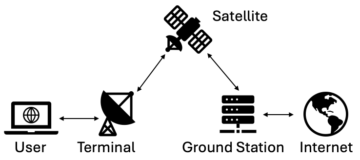
are terrestrial gateways that bridge the Starlink satellite network to the broader terrestrial Internet infrastructure. Satellites relay traffic received from terminals to a ground station, which routes data to its final Internet destination using terrestrial connectivity. Figure 2 summarizes the complete Starlink ecosystem, including user terminals, ground stations and satellites.
3 Impact of Obstructions
Starlink connectivity is crucial for environments lacking traditional terrestrial broadband infrastructure, like wildfire detection outposts deep within forests and emergency communication sites in disaster-struck regions. However, terminals in these settings are frequently subject to physical obstructions. Dense forest cover, debris, or other natural barriers may obstruct the line-of-sight (LOS) path between terminals and satellites, potentially impairing connectivity. Despite the practical significance of these scenarios, the impact of physical obstructions on satellite connectivity and performance remains under-explored. We address this gap through controlled experiments that systematically assess how obstructions affect Starlink connectivity.
Experimental hardware setup.
We deploy a testbed consisting of two identical Starlink user terminals on the roof of a three-story building in NY state. Both terminals use the standard Starlink hardware [8] and subscribe to the Residential service plan. To ensure an accurate baseline comparison, both terminals initially have an unobstructed view of the sky, free from trees, buildings, or other barriers (§4). One terminal acts as the test device, which we subject to controlled obstructions, while the other is a control device for providing baseline connectivity and performance metrics.
Ensuring similar test vs. control conditions.
We co-locate the terminals approximately six feet apart, ensuring they have nearly identical views of the satellite constellation, while still being far enough apart that the obstructions applied to the test dish do not affect the control dish. Both dishes are oriented towards the northeast direction following recommendations from the Starlink mobile application. Throughout the experiment, we use the application’s obstruction visualization feature to confirm that introduced obstructions only impact the test terminal, leaving the control terminal unobstructed. This carefully controlled setup allows us to clearly isolate and measure the impact of obstructions on performance of the test dish.
Types of obstructions studied.
We experiment with two types of obstructions that represent realistic field scenarios:
-
Line-of-Sight Obstruction. We use a galvanized steel metal sheet, measuring 30 inches wide by 25 inches tall, to obstruct specific areas of the sky from the perspective of the test terminal (Figure 1(a)). This controlled obstruction setup simulates LOS barriers like dense foliage or physical structures that may partially or fully block satellite visibility. Following FCC guidelines [5] which specify a minimum operational elevation angle of 25 degrees from the dish, we position the metal sheet at varying distances and elevate it to 14 inches above ground level using a stable stand. This approach of obstructing the control dish enables precise control and repeatability of experiments. Galvanized steel effectively blocks electromagnetic radiation, preventing satellite signals from passing through the obstructed area [49]. We validated this shielding effect experimentally by fully covering the dish with the metal sheet, observing that it prevented all satellite connections and kept the terminal disconnected.
-
On-Top Obstruction. To simulate the effect of debris accumulation directly on the terminal, we place a black aluminum foil onto the dish surface (Figure 1(b)). We systematically vary the size and position of the foil to evaluate how different degrees of partial dish obstruction impact connectivity and performance.
Rationale for using a metal sheet as obstruction.
We chose to evaluate the effect of obstructions on satellite connectivity using a metal sheet that can be positioned at different distances from the control dish. Our rationale for this obstruction setup is that it allows us to have precise control and repeatability in the experiment. The metal sheet emulates the obstructive effects of real-world barriers while maintaining a simple geometric shape. While real-world obstructions, like trees, buildings, or debris, have irregular shapes that lead to variable signal attenuation characteristics, they are difficult to reposition accurately and consistently. In contrast, the metal sheet allows precise and repeatable obstruction placement, enabling systematic evaluation of obstruction effects on Starlink connectivity. Although real-life obstructions are more complex, the controlled nature of our metal sheet experiments allow us to isolate effects that would be challenging to attribute solely to obstructions if natural barriers (e.g.,trees and vegetation) were used.
Related insights from electromagnetic research.
Previous studies on electromagnetic interference and satellite communication have helped in devising our measurement strategy as well as provide useful context for interpreting our results [13, 14, 38]. Related research highlights how electromagnetic shielding materials like galvanized steel effectively attenuate satellite signals, validating our methodological choice of using a metal obstruction to simulate LOS barriers [49]. Additionally, studies of phased-array antenna technology in LEO satellite systems underscore how dynamic beam steering can mitigate obstructions, a relevant consideration when interpreting our experimental results. We have integrated these insights from literature on electromagnetic radiation to position our controlled obstruction experiments within a broader technical context.
Timeline of experimentation.
We originally established the hardware setup and initiated the measurement campaign in July 2024. However, several potential physical locations proved unsuitable due to existing natural obstructions like houses and tall trees. In October 2024, we relocated the testbed to the rooftop of a three-story building, ensuring both terminals had unobstructed views, thus enabling systematic evaluation of obstruction-induced performance impacts.
4 Measurement Methodology
We establish wired Ethernet connections between each Starlink terminal (Figure 1) and dedicated mini-PCs through the dish’s router in bridge mode. We use Ethernet instead of default wireless to avoid interference and ensure reliable connections. Both mini-PCs have identical specifications (Intel N95, 8GB RAM, 256GB storage) and Ubuntu 22.04.
The mini-PCs run measurement tools to continuously gather performance metrics to a dedicated server in central US, collecting latency, packet loss, and obstruction maps. We backup data every 10 minutes via out-of-band channels to minimize risk of data loss and use distinct network namespaces to isolate measurement and data collection traffic.
4.1 Baseline test vs. control comparison
With both dishes unobstructed, we measure fine-grained RTT from each terminal to our measurement server using iRTT [2] at 20 ms intervals. Figure 3(a) shows hourly median RTT over 10 days, we can observe similar aggregate latency for both dishes. The tail latencies ( and percentiles) also exhibit similar distributions.
Loss.
We calculate packet loss percentage defined as the fraction of lost packets during a specific time interval using lost packets from RTT measurements over 1-hour intervals for 10 days (Figure 3(b)). The positive y-axis shows control dish loss and negative y-axis shows test dish loss. Both dishes perform similarly with occasional high loss spikes between 12AM-4AM (most frequently at 3AM), likely due to Starlink infrastructure maintenance rather than user traffic.
4.2 Identifying the serving satellite
Having confirmed both dishes perform similarly under unobstructed conditions, we next evaluate if they connect to the same satellite given their identical environment, location, and hardware. Since Starlink’s software does not reveal which satellite a dish connects to among thousands available, we develop a rigorous methodology to identify the terminal-to-satellite mapping. This mapping is time-varying with satellite hand-offs occurring every fifteen seconds.
Recent work has undertaken this challenge and our work builds on their techniques while improving the accuracy and verifying the mapping with other techniques [44, 12]. In essence, our method compares the trajectory of the connected satellite, obtained using the Starlink-gRPC [6] API, to publicly available satellite trajectory data from Celestrak [1]. This comparison must be done carefully to prevent spurious matches. We summarize our complete algorithm for the comparison in Figure 5. In this section, we describe the complete satellite identification algorithm.
Gather trajectory of the connected satellite.
We use the Starlink-gRPC API to obtain a 2D obstruction map (123px 123px grid) capturing satellite movement. While the Starlink mobile application provides 3D visualization, only the 2D version is programmatically accessible. Figure 4(b) shows an obstruction map from the API where white pixel-based lines represent satellite trajectories, continuously updated as satellites move with each pixel representing satellite position relative to the dish.
Resetting maps.
Over time, overlapping satellite trajectories crowd the obstruction map, making satellite identification challenging. We address this by clearing the map every minute using the Starlink-gRPC API, choosing a one-minute window to avoid frequent resets while allowing time to start trajectory repopulation. Since satellite handovers occur at 12, 27, 42, and 57 seconds, we reset at 56th second to maximize captured trajectory data with 1 second for processing.
Fast map reset.
During each reset cycle, we capture snapshots every 15s at 11, 26, 41, and 56 seconds, timed one second before expected handover events for processing delays. While related work reboots dishes every 10 minutes, the Starlink-gRPC reset API enables map clearing without rebooting, capturing trajectory data with reduced overlapping trajectories [44].
Isolating the trajectories.
Since the trajectory is continuously populated on the same map, isolating the most recent trajectory (i.e.,the trajectory populated during the last 15 seconds between and snapshot) from snapshot of the obstruction map requires additional processing. Following the approach of [44] for isolating the trajectory, we compute an XOR between the and the snapshot captured for the previous 15 second window.
Dealing with residual trajectories.
XOR alone can leave residual trajectories from previous resets. We address this by applying an additional AND operation between the snapshot and XOR result, filtering outdated points to retain only the most recent trajectory from the snapshot. Figures 4(b)-4(e) show the snapshots and operations where XOR retains trajectories from both snapshots while AND isolates the most recent trajectory.
Mapping the trajectory to a satellite.
To map the trajectory to a satellite, we first convert the trajectory data to a format compatible with public satellite information. Satellite positions in Celestrak are represented using azimuth and angle of elevation (AOE) [23], as shown in Figure 2. For each trajectory, we compute the AOE and azimuth per pixel. Since the obstruction map uses a polar coordinate system, AOE is estimated based on the radial distance from the center of the map, while azimuth is determined by measuring the clockwise angle from the top (North) of the map [44, 6].
Dynamic Time Warping.
We compare extracted trajectories to Celestrak satellite data [1] for identification. Since Celestrak updates only every six hours, we use SGP4 [47] to compute real-time satellite positions. We find the best match between the obstruction map and public satellite data we use Dynamic Time Warping (DTW) distance [42], and classify the satellite with smallest DTW distance as the serving satellite. For computing DTW distance, both trajectories are converted from polar to Cartesian coordinates using and , where is radial distance or azimuth and is AOE.
4.3 Accuracy of satellite matching
Using our satellite identification algorithm (Figure 5), we find that both test and control dishes were connected to the same satellite over 97% of the time. Given their close physical placement (6 feet apart) and the similarity in their observed performance, high overlap in connectivity is unsurprising. However, in cases where the algorithm classified the dishes as connected to different satellites, we analyzed the obstruction maps and found that the extracted trajectories from test and control dishes were nearly identical. However, minor variations in trajectory data led to misclassifications.
Top-k satellites.
To address misclassification, we consider the k closest satellites based on DTW distance, rather than relying solely on the single closest match. By analyzing the top k candidates, we can account for minor variations in trajectory data. With k=2, we find that both dishes connect to the same satellite over 99.9% of the time, confirming that the observed mismatches resulted from minor trajectory variations. We compare the trajectories directly next to further validate the results.
DTW distance based trajectory comparison.
Rather than mapping trajectories to a satellite and then comparing the matched satellites, we directly compare the trajectories from both dishes using difference in DTW values. We convert the polar coordinates to Cartesian coordinates for comparison.
AOE or r can vary from 25 to 90, on the other hand azimuth can vary from 0 to 360 degrees but converting to Cartesian coordinates involves taking or of azimuth which limits its values between 0 and 1. This causes the DTW distance to vary widely with changes in r but not with . To account for this, we normalize r using multiple methods to bound the value between 0 and 1 and compare the results. We normalize r by the following methods: 1. dividing by maximum value of r (90), 2. normalizing over the range of 25 to 90, 3. taking , and 4. taking . The equations for these normalization methods are shown below.
| (1) |
Using the normalized values of r, we compute the difference in DTW distance between the two trajectories. Figure 6 shows the DTW distance for the default non-normalized value of r has a knee around 0.97. In contrast, all other normalization methods show the knee around 0.99. This suggests that even without normalization, the DTW distance between the control and test trajectories is very low, indicating strong similarity. After normalization, the DTW distance decreases even further, reinforcing that the trajectories are highly similar and the dishes are connected to the same satellite.
Takeaway: Both the dishes are connected to the same satellite over 97% of the time.
4.4 Connection region
We analyze the satellite connection region relative to the terminal to evaluate the impact of orienting the terminal in the northeast direction, as suggested by the Starlink mobile application. This analysis will also inform our strategies for obstruction placement. As established in Section 4.2, both terminals are connected to the same satellite over 97% of the time so we analyze the connection region for one terminal. We present results for the control terminal (since both terminals exhibit similar connection region). Figure 7 plots the azimuth and AOE for January 29 and January 30; additional days show similar trends but are omitted for clarity. The terminal primarily maintains connections within an azimuth range of 50°–150° and an elevation range of 25°–90°. The observed elevation range aligns with FCC filings [5], which specify a minimum operational elevation of 25°. The azimuth range suggests that the terminal primarily connects to satellites in the east, northeast, and southeast directions. These connection characteristics remain consistent across the entire experiment for both terminals.
5 Starlink under obstruction
In the previous section (§4) we established that in the absence of obstructions, both terminals connect to the same satellites over 97% of the time. Moreover, they primarily connect to satellites in the north-east, east and south-east directions of the sky. In this section we explore the obstruction’s impact on connectivity and performance of terminals.
5.1 Profiling the obstructed region
To recreate LOS obstruction, we positioned a metal sheet to obstruct the test terminal. Using trigonometry, we estimated the blocked sky region using computed AOE and azimuth based on obstruction size and distance from the dish. We validated estimates against the Starlink obstruction map by confirming the blocked AOE, azimuth, and direction:
Estimating the blocked AOE.
Using obstruction height and distance from the dish as shown in Figure 4(a), we estimated the blocked AOE, which closely matched the obstruction map. We validated results by testing different distances.
Estimating the blocked azimuth region.
Using obstruction width and distance, we estimated blocked azimuth. Initial results showed a 1.5x offset, which we adjusted for in further calculations. We validated the adjusted model by testing different distances and directions and found alignment with the obstruction map.
Estimating obstructed direction.
We estimated the obstructed direction using easily available devices, including a mobile phone compass, an orienteering compass, and a smartwatch compass. However, these devices yielded inconsistent results. To align with the obstruction map, we adjust the direction by referencing the Starlink obstruction map.
After validating our estimates and accurately profiling the blocked region, we examine the directional impact of the obstruction placement, leveraging the observation that the dish predominantly connects in specific directions.
5.2 Impact of obstructed direction
To analyze the effect of obstructed direction, we placed the obstruction at 44 inches from the terminal as shown in Figure 4(a) to block a reasonable part of the sky. As both terminals faced 40 northeast, we tested four orientations for the obstruction: northeast (NE), northwest (NW), southeast (SE), and southwest (SW). The obstruction was placed symmetrically and parallel to the terminal’s closest edge. Each configuration was maintained for 3 days to allow the obstruction map to be populated.
North-East direction.
The obstructed area appeared clearly, indicating that the dish experienced obstruction in its LOS, as shown in Figure 8(a). This aligns with our expectations, as the dish primarily connects to satellites in the eastern region. Despite the obstruction in the connection area, we did not observe a significant RTT or loss degradation.
South-East direction.
The obstructed area appeared clearly as shown in Figure 8(c). This aligns with our expectations based on the connection region. In this case, the obstruction led to 4% increase in RTT on average for the test dish compared to the control dish. We also observed an average increase from 0.1% to 0.4% in packet loss.
North-West direction.
South-West direction.
The obstruction did not appear in the obstruction map and no performance degradation was observed, as it was located behind the dish where satellites are not typically accessed.
Hence, we can say that the obstruction’s impact depends on the direction it is placed in. Obstructions in SE degraded performance the most, followed by the obstruction in NE. On the other side, obstructions in the NW and SW directions had minimal impact on the dish’s performance. Given that the obstruction in the SE direction had the most impact on performance, we further investigated this direction to better understand the causes of performance degradation.
To understand the performance impact of obstructing the south east region, we measured RTT and packet loss following the methodology outlined in §4. Figure 9(a) shows the hourly median RTT over a 10-day period to assess aggregate performance along with the tail latencies ( and percentiles) of both dishes. We observe that the obstructed (test) terminal observes a persistent RTT increase of approximately 4% on average compared to the control dish. Similarly, we calculate the percentage of packet loss over 1-hour intervals and tail latencies for the same 10-day period. Figure 9(b) shows consistently higher loss with an absolute increase of 0.3% in presence of the obstruction.
Satellite identification.
Using the satellite identification method described in §4, we calculate the percentage of instances where the test terminal connected to a different satellite than the control terminal.
We observed that the test terminal connected to a different satellite in 15% of the cases on average for SE. The daily percentage of such connections are shown in Figure 10. This indicates that the obstruction in affected the satellite connection area and led to a different satellite being selected.
Takeaway: Under obstructed conditions, the test dish has 4% higher RTT and 0.3% higher packet loss compared to the control dish and connects to different satellites in about 15% of the cases on average.
Change in connection area.
We observed changes in the connection area of the test dish as shown in Figure 11 using cumulative distribution function (CDF) rather than using a scatter plot as in Figure 7, as the scatter plot makes it difficult to present these changes. The CDF reveals that the test terminal’s azimuth shifted north to avoid the obstructed area (marked with gray lines), while the control terminal also unexpectedly changed its connection area.
Obstruction leakage.
As shown in Figure 11, in the unobstructed scenario, the azimuth CDF of both the terminals overlapped as expected. In the obstructed scenario, we anticipated the control terminal’s CDF to remain unchanged and aligned with the unobstructed case. However, we observed a slight shift in the control terminal’s azimuth distribution toward the north, despite no visible obstruction in its obstruction map. To verify whether this shift was caused by the obstruction placed for the test terminal, we removed the obstruction and found that both the terminal’s azimuth distribution returned to its original pattern. This suggests two possible scenarios: (1) the obstruction may have partially interfered with the control terminal’s line of sight despite not being registered in the obstruction map, or (2) the obstructed test terminal indirectly influenced Starlink’s satellite selection algorithm, causing the control terminal to change its connection area. If the latter is true, it indicates a vulnerability in the connection algorithm of Starlink which can be exploited to affect the connectivity of other terminals.
These results confirm that obstructions in critical connection regions directly impact connectivity and performance.
Obstruction in the east direction.
When the obstruction was placed in the east direction, we observed performance similar to the southeast direction. Since the dish connects in this general direction, the results were expected. Interestingly, the connection area shifted towards south, unlike southeast direction, where it shifted towards the north. This points that the dish often connects between east and south east directions.
Effect of distance.
We initially placed the obstruction at a distance of 44 inches from the dish. To assess the impact of distance, we moved the obstruction closer which resulted in an increase in the blocked azimuth range and reduction in blocked AOE range due to the elevation of the obstruction as shown in Table 1. As the distance decreased, we observed improvements in both RTT and loss. At 42 inches the performance was comparable to the control dish, suggesting that the dish handles blocked azimuth better than blocked AOE.
| Distance (in) | Blocked Az. Range () | Blocked AOE Range () | Blocked Az. Dist. () | Blocked AOE Dist. () |
| 44 | 58.4–111.6 | 37–58.1 | 53.2 | 21.1 |
| 43 | 55–115 | 41.6–60.3 | 59.8 | 18.7 |
| 42 | 50.6–119.3 | 48.3–62.8 | 68.7 | 14.5 |
Performance at the edge of obstruction.
In practice, when the LOS between the dish and its serving satellite is near the boundary of the blocked region, the dish can often remain connected, but performance begins to degrade. As the LOS moves further into the blocked region, RTT and packet loss tend to degrade, until the dish eventually loses connectivity as shown in Figure 12.
On-terminal obstruction.
We studied the on-terminal obstruction scenario by placing a thin aluminum sheet on top of the dish to simulate the accumulation of debris as shown in Figure 1(b). When the dish was fully covered, it was unable to connect to any satellite. However, when half of the dish was covered, it successfully established a connection and showed no performance degradation in terms of loss and latency. This shows that the dish can tolerate partial on-terminal obstructions.
6 Response to obstructed dishes
In the previous section, we demonstrated how obstructions have a tangible negative effect on the network performance of user terminals. However, despite being severely obstructed, the test user terminal maintains network connectivity, albeit with reduced performance. This shows a high degree of resilience in the Starlink infrastructure. While empirically studying this resilience, we identify a mechanism using which the Starlink ecosystem achieves this resilience. We call this mechanism responsive routing.
Responsive routing.
We find empirical evidence of cases when both the obstructed and unobstructed terminals connect to the same satellite in a 15 second time slot. However, during this time slot, the obstructed dish switches to a different satellite compared to the one it originally connected to. We argue that this effect reveals that the Starlink ecosystem has enabled user terminals to respond to poor performance (i.e.,potentially obstruction induced) outside of the usual fifteen-second scheduling loop that typically maps terminals to satellites. In this section we examine the evidence of responsive routing by first establishing that (1) the test terminal connects to two different satellites within the 15-second time slot (§6.1) and (2) the test and control terminals first connect to the same satellite at the beginning of the time slot (§6.3).
6.1 Evidence of responsive routing
We observe that in some obstruction scenarios, the test dish connects to different satellites than the control dish about 15% of the time. During these connection windows, the test dish observes many packet loss spikes. This suggests that the test dish is experiencing a significant obstruction in the LOS to the satellite, leading to disruption in connectivity. In such instances, the test dish may switch to a different satellite to maintain connectivity. Based on the data collected over 11 days between 4th January 2025 and 14th January 2025, we present our observations about this phenomenon:
Partial satellite trajectories.
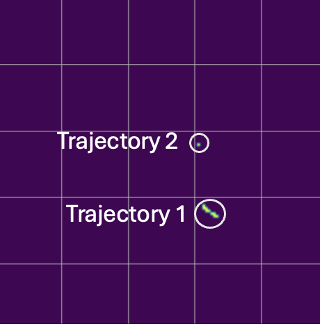
In some time windows when the test dish connects to a different satellite compared to the control dish, we observe partial trajectories in the obstruction map of the test dish as shown in Figure 13(a). We observe two distinct trajectories, trajectory 1 in color blue for the obstructed region and trajectory 2 in green for the clear region. We call the trajectory that is not the longest trajectory in such cases, as an extra partial trajectory.


Mid-slot handovers.
As per this observation, there are cases when the test dish switches the satellite connection during the slot, contrary to the popular belief that handovers happen only at the end of a 15 second slot [44]. Note that even when the satellite changes mid-slot, the usual handover still occurs at the end of the 15-second slot. These mid-slot switches are accompanied by high packet loss, suggesting that the dish changes satellites in response to the obstructions. Figure 12 shows an example of this behavior where the obstructed dish connects to a satellite at , experiences high loss and latency, and switches to a different satellite around within the same 15-second slot. Figure 13(a) shows the corresponding obstruction map, with Trajectory 1 and Trajectory 2 representing the initial and subsequent connections. In contrast, the control dish remains connected to the same satellite as shown in Trajectory 1 in Figure 13(b), while Trajectory 2 shows the underflow behavior described in Section §6.2. We observe partial trajectories like Trajectory 2 in the obstruction maps of the test dish approximately 6% of the time compared to just 0.3% for control dish. We discuss this difference later in the section.
Single pixel partial trajectories.
The partial trajectory can be as short as a single pixel in the obstruction map, which would occur when the connection is very brief, resulting in fewer pixels being populated in the obstruction map. When the connection is too short, the trajectory may not be visible on the obstruction map, unfortunately preventing us from identifying such cases as instances of responsive routing.
6.2 Explaining away responsive routing
In this section, we try to consider alternate hypotheses that might explain or negate our responsive routing hypothesis. A potential explanation for partial trajectories is that the trajectory on the map could be an overflow or underflow from the 15 second connection window as shown in Figure 14. We categorically eliminate cases of overflow and underflow to check if evidence of responsive routing still exists. We use pixel and partial trajectory interchangeably in this section.
Time windows.
To understand pixel overflow and underflow we name connection windows. The currently examined 15s connection window for pixel identification and classification is the current window. The 15s window right before the current window is previous window and the window right after the current window is next window. Figure 14 shows the underflowed pixel in the current window 14(a) since it matches the trajectory from the next window 14(b). This occurs when the trajectory data is captured right after the handover. Similarly, we can have a pixel overflow where the pixel in the current window is populated from the next window’s trajectory data which can happen when the trajectory data is captured right before the handover.
Causes of overflow/underflow.
The pixel overflow or underflow can occur due to the data capturing process. Since the trajectory data is captured just 1 second before the handover, processing delays may cause some pixels in the obstruction map to overflow or underflow the 15s connection window. For such a disjoint pixel in the obstruction map of the current window, we identify the following scenarios:
-
Underflow. If the disjoint pixel in the current window is populated from the next window, we identify it by checking the trajectory in the next window. If it matches the trajectory, within a threshold defined as the maximum allowable pixel distance between two trajectory points for overflow or underflow, we classify it as an underflow.
-
Overflow. If a pixel in the current window is from the trajectory in previous window, we can identify it by checking the trajectory in the previous window.
-
Neither. If the pixel is neither overflowed nor underflowed (i.e.,populated in the current window) then we classify the pixel as a distinct trajectory and therefore as evidence of responsive routing.
For identifying evidence of disjoint routing, we do not consider cases where a pixel in the current window could have overflowed or underflowed into the previous or subsequent window. Instead, we specifically address and exclude scenarios where pixels in the current window have originated (overflowed or underflowed) from neighboring windows. This approach is necessary because it is uncertain whether pixels originating from adjacent windows correspond to a different satellite connection during the current observation window. If a pixel has overflowed or underflowed into adjacent windows and aligns with the trajectory in the current window, we conclude it is from the same satellite connection. If it does not match, we cannot determine if it overflowed or underflowed.
Table 2 summarizes the pixel populating scenarios for the test and control dishes. It splits connection windows into four categories: (1) no extra trajectory, when only one trajectory is seen; (2) extra trajectory, when multiple trajectories are present but neither overflow nor underflow occurs; (3) underflow, when the pixel in the current window originated from the next window; and (4) overflow, when the pixel in current window originated from previous window.
Table 2 illustrates these pixel populating scenarios across three different threshold values (0, 1, and 2). The threshold value influences trajectory classification into overflow and underflow. At threshold 0, the trajectory must precisely overlap with adjacent window trajectories, an unlikely condition due to satellite motion dynamics. Increasing the threshold to 1 reduces extra trajectory occurrences from 19.64% to 0.37% for the control dish and from 22.66% to 6.38% for the test dish. We attribute this reduction to increases in underflow and overflow. These results indicate that the test dish frequently connects to multiple satellites within the 15-second connection interval due to obstructions. Increasing the threshold further to 2 does not significantly alter the results, confirming that a threshold value of 1 is adequate.
Table 2 and Table 3 present the pixel populating scenarios. Table 3 specifically focuses on instances when the satellite identification algorithm determined the dishes connected to different satellites. In these cases, the extra trajectory scenario accounts for 21.28% for the test dish but only 0.66% for the control dish, reinforcing that the test dish has a higher chance of connecting to multiple satellites in obstructed connection windows.
| Threshold | Terminal | No Extra Trajectory (%) | Extra Trajectory (%) | Underflow (%) | Overflow (%) |
| 0 | Control | 80.21 | 19.64 | 0.11 | 0.02 |
| 0 | Test | 73.26 | 22.66 | 3.13 | 0.97 |
| 1 | Control | 80.21 | 0.37 | 17.15 | 2.24 |
| 1 | Test | 73.26 | 6.38 | 16.63 | 3.74 |
| 2 | Control | 80.21 | 0.32 | 17.24 | 2.21 |
| 2 | Test | 73.26 | 6.02 | 16.85 | 3.88 |
| Threshold | Terminal | No Extra Trajectory (%) | Extra Trajectory (%) | Underflow (%) | Overflow (%) |
| 0 | Control | 75.22 | 24.64 | 0.17 | 0.04 |
| 0 | Test | 40.04 | 49.88 | 6.12 | 3.95 |
| 1 | Control | 75.22 | 0.66 | 22.61 | 1.59 |
| 1 | Test | 40.04 | 21.28 | 27.42 | 11.32 |
| 2 | Control | 75.22 | 0.62 | 22.69 | 1.53 |
| 2 | Test | 40.04 | 20.00 | 27.71 | 12.23 |
Takeaway: In about 21% of satellite connections when classified as connected to different satellites, the obstruction map of the test dish shows an extra trajectory, indicating that it connected to a different satellite than the control dish during the same 15-second interval.
6.3 Same initial satellite allocation
We found partial trajectories in the obstruction map of the obstructed dish. These partial trajectories result from connecting to different satellites during the 15-second connection window. We found that the partial trajectory in the obstruction map of the test dish overlaps with the trajectory of the control dish, as shown in Figure 13 where Trajectory 1 from the obstruction map of the test dish (Figure 13(a)) matches the trajectory in the obstruction map of the control dish (Figure 13(b)). This suggests that the test dish initially connected to the same satellite as the control dish but then switched away due to obstruction.
In the evaluation of responsive routing, we only considered overflowed from or underflowed from cases for the current window but now we can consider the overflowed to and underflowed to cases and evaluate the partial trajectories in adjacent windows as well. This is because we can match the partial trajectory with trajectory from control dish and verify. To handle both to and from cases, we need to consider all three scenarios (overflow, underflow, and neither) for each window (previous, current, and next).
First, we take a look at the pixel in the current window of the test dish for all the pixel populating scenarios. If classified as either overflow or underflow, we do not consider it for the evidence of the test dish first connecting to the same satellite as the control dish.
-
Overflow. We again use the method used in §6.1 to check for overflow. If the pixel in the previous window is in the same location as the pixel in current window within threshold, we classify the pixel as overflow.
-
Underflow. Underflow can be identified by checking the test dish trajectory of the next window. If underflowed, we dont consider it for evidence of the test dish first connecting to the same satellite as the control dish.
-
Neither. If the pixel is neither overflowed nor underflowed then we compare the trajectory in the current window of the control dish. If matching, we classify the pixel as evidence of the test dish first connecting to the same satellite as the control dish.
Second, we look at the pixel in the previous window of the test dish for all the pixel populating scenarios.
-
Overflow. Pixel in the previous window is populated from the previous window of the previous window (previous previous window). This can be identified by checking the test dish trajectory of the previous previous window and if the pixel is in the same location within threshold as the pixel in previous window, we classify as overflow.
-
Neither. The pixel in the previous window is populated during the previous window. This can be identified by checking the control dish trajectory of the previous window. If the pixel in the previous window is within threshold, we classify the pixel as belonging to the previous window and not consider it.
-
Underflow. The pixel in the previous window is populated from the next (i.e. current) window. For underflow, we first need to check if the pixel is underflowed from the longest trajectory in the current window. This can be identified by checking the test dish trajectory of the current window. If the pixel in the current window is in the same location within threshold as the pixel in previous window, we classify the pixel as underflow from longest trajectory and not consider it. But if the pixel is not underflowed from the longest trajectory, we compare it with the trajectory of the control dish for the current window. If satisfied, we classify the pixel as evidence of the test dish first connecting to the same satellite as the control dish.
Finally, we look at the pixel in the next window of the test dish. The pixel from the current window can be populated into the next window only in the overflow scenario. However, even if this occurs, it would be from the last satellite connection in the current window, which cannot serve as evidence that the test dish initially connected to the same satellite as the control dish. Therefore, we do not need to consider pixel population scenarios in the next window.
| Threshold | Same Satellite (%) | Different Satellite (%) | No Trajectory (%) | Other (%) |
| 0 | 38.56% | 12.37% | 29.37% | 18.70% |
| 1 | 24.98% | 4.89% | 37.88% | 43.74% |
| 2 | 23.53% | 4.87% | 38.09% | 44.69% |
For evaluation we only consider scenarios where the satellite identification algorithm classified the dishes as connected to different satellites. Table 4 shows the pixel classification for the test dish when first connected to the same satellite as the control dish before moving away. We evaluate for 3 thresholds and results again stabilize at threshold of 1. We see that 25% of the time, the test dish connected to the same satellite as control dish, close to 5% of the time the test dish connected to a different satellite and about 38% of the time, there was no extra trajectory visible in the obstruction map. Note that this could happen due to the brief nature of the connection and consequently the pixel not being populated. The remaining 43% of the time includes all the other scenarios such as overflow and underflow from both the previous and current window as described above.
| Threshold | Same Satellite (%) | Different Satellite (%) | No Trajectory (%) |
| 0 | 42.31% | 24.80% | 23.33% |
| 1 | 67.31% | 17.39% | 22.25% |
| 2 | 67.72% | 17.01% | 22.13% |
If we do not give overflows and underflows higher precedence than the same satellite case and thus relax the pixel classification as shown in Table 5, we see that about 67% of the time, the test dish connected to the same satellite as control dish. Around 17% of the time, it connected to a different satellite, and about 22% of the time, no additional trajectory was visible in the map.
Takeaway: Over 67% instances, both dishes initially connect to the same satellite before the obstructed dish switches the satellite under relaxed classification.
6.4 Performance impact
Responsive routing aims to mitigate loss of connectivity from scenarios of poor performance, including but not limited to severely obstructed user terminals. We find that even with such routing, the obstructed dish observes worse performance relative to the control dish due to the increased latency during satellite switches. Figure 15 shows the CDF of median and p05 ( percentile) latency differences per connection window, grouped by whether the obstructed dish connects to the same or a different satellite than the control dish. When connected to different satellites due to responsive routing, the test dish exhibits higher median latency in about 70% of cases. Moreover, the latency increases are larger in magnitude than any improvements. Since median RTT may be affected by transient spikes during satellite switching, we also report the p05 latency, which shows a similar trend.
7 Related work
LEO characteristics and measurement Studies.
Recent measurement studies have provided valuable insights into the performance of LEO satellite networks, particularly Starlink. [37] restricts the terminal’s field of view using an obstruction to force it to connect to specific satellites and enable a better understanding of satellite handoff and connectivity. However, it does not analyze responsive routing or performance characteristics during the transition from obstructed to unobstructed regions in controlled experiments. Several works have focused on performance from the end-user perspective [35, 36, 46], conducted large-scale measurement studies [37], and examined performance variability across geographic regions [30, 18], while also proposing improvements [39]. Other studies have investigated component-specific performance, such as access link behavior and the impact of edge routers [40, 24]. [20] explores Starlink’s potential and challenges as a global ISP. Since providers do not expose endpoints to identify the serving satellite, some works have inferred this information using satellite trajectories and publicly available data [44, 12]. Additionally, several studies have evaluated Starlink’s video streaming performance and proposed algorithms to enhance it [27, 10, 50]. Similar measurement efforts have also been conducted for GEO satellite networks [41]. To the best of our knowledge, no prior work has specifically focused on the performance of Starlink under obstructed conditions. Our work aims to fill this gap by providing a comprehensive analysis of Starlink’s performance in both obstructed and unobstructed scenarios.
LEO network design and architecture.
Prior work has focused on network topology, routing protocols, and design to improve latency and capacity [16, 22, 25]. While some systems rely on inter-satellite links [16] for routing, others have explored ground stations for forwarding [26, 48] and developed scheduling strategies to manage satellite-to-ground traffic effectively [45]. Due to unique nature of LEO traffic, researchers have explored congestion control over LEO networks [29] and have proposed interesting applications [17] and the potential challenges of LEO networks [15]. To improve the performance of LEO networks, several works have proposed better beamforming methods with DNN for ground stations [31] and better handover methods for LEO satellites [28, 33]. Security researchers have also explored various aspects of LEO network security [21, 43]. Our work provides a unique perspective on the behavior of Starlink under obstructed conditions and provides insights into the handover process along with evidence of responsive routing.
Satellite connectivity in remote environment.
8 Limitations and Future Work
-
Our study focuses on deployment of Starlink terminals in New York (US), where the terminals primarily connect to satellites in the eastern sky. This dominant direction of connectivity can vary with location of terminals, so our results may differ at other latitudes and longitudes. However, we believe that the mechanism of responsive routing is a general one employed by Starlink to maintain connectivity and is not specific to our deployment.
-
To control obstructions precisely, we use a metal sheet to block specific regions of the sky. This approach does not fully capture the irregular shapes and partial attenuation of real-world obstructions like trees or buildings. However, it allows us to isolate the effect of directional obstruction in a repeatable way. Future work can extend this analysis to more diverse geographies and incorporate more realistic obstructions to better reflect real-world scenarios.
9 Conclusion
We present a comprehensive study of the impact of physical obstructions on Starlink connectivity using a controlled two-terminal testbed. Without obstructions, both terminals show similar performance and connect to the same satellite over 97% of the time. By introducing obstructions to the test terminal, we found that obstruction in specific areas could affect the overall performance and connectivity of the terminal. We observe that Starlink’s routing system dynamically adapts to obstructions by switching the affected terminal to a different satellite in real time. In many cases, both terminals initially connect to the same satellite, but the test terminal switches to a different one due to the obstruction. Overall, our work provides valuable insight on the connectivity and performance of Starlink under obstructed conditions, which is crucial for understanding the challenges of deploying LEO satellite networks in real-world scenarios.
References
- [1] Celestrak. URL: https://celestrak.org.
- [2] Irtt. URL: https://github.com/heistp/irtt.
- [3] Project kuiper. URL: https://www.aboutamazon.com/what-we-do/devices-services/project-kuiper.
- [4] Starlink dish specifications. URL: https://www.starlink.com/specifications.
- [5] Starlink fcc 21 report. URL: https://docs.fcc.gov/public/attachments/fcc-21-48a1.pdf.
- [6] Starlink-grpc-tools. URL: https://github.com/sparky8512/starlink-grpc-tools.
- [7] Starlink media kit. URL: https://www.spacex.com/media/starlink_media_kit_jan2020.pdf.
- [8] Starlink specifications. URL: https://www.starlink.com/specifications?spec=4.
- [9] Starlink updates. URL: https://www.starlink.com/updates.
- [10] Toward robust live streaming over leo satellite constellations: Measurement, analysis, and handover-aware adaptation. URL: https://api.semanticscholar.org/CorpusID:273903447.
- [11] Types of orbits. URL: https://www.esa.int/Enabling_Support/Space_Transportation/Types_of_orbits.
- [12] Ali Ahangarpour, Jinwei Zhao, and Jianping Pan. Trajectory-based serving satellite identification with user terminal’s field-of-view. In LEO-NET, 2024. URL: https://api.semanticscholar.org/CorpusID:273550364.
- [13] Giandomenico Amendola, Daniele Cavallo, Tobias Chaloun, Nicolas Defrance, George Goussetis, Marc Margalef-Rovira, Enrica Martini, Oscar Quevedo-Teruel, Vaclav Valenta, Nuno J. G. Fonseca, and Mauro Ettorre. Low-earth orbit user segment in the Ku and Kaband: An overview of antennas and RF front-end technologies. IEEE Microwave Magazine, 24(2):32–48, 2023. doi:10.1109/MMM.2022.3217961.
- [14] Yanki Aslan and Antoine G. Roederer. Multiple beam forming schemes for user terminal antennas: Now and next. In Stefania Monni and Enrica Martini, editors, Reviews of Electromagnetics, Vol. III: Antenna Systems for Satellite Communication Terminals, volume 3, pages 4–26. Reviews of Electromagnetics, 2024. doi:10.53792/roe/2024/23004.
- [15] Debopam Bhattacherjee, Waqar Aqeel, Ilker Nadi Bozkurt, Anthony Aguirre, Balakrishnan Chandrasekaran, P. Brighten Godfrey, Gregory Laughlin, Bruce Maggs, and Ankit Singla. Gearing up for the 21st century space race. In Proceedings of the 17th ACM Workshop on Hot Topics in Networks, HotNets ’18, pages 113–119, New York, NY, USA, 2018. Association for Computing Machinery. doi:10.1145/3286062.3286079.
- [16] Debopam Bhattacherjee and Ankit Singla. Network topology design at 27,000 km/hour. In Proceedings of the 15th International Conference on Emerging Networking Experiments And Technologies, CoNEXT ’19, pages 341–354, New York, NY, USA, 2019. Association for Computing Machinery. doi:10.1145/3359989.3365407.
- [17] Vaibhav Bhosale, Ada Gavrilovska, and Ketan Bhardwaj. Krios: Scheduling abstractions and mechanisms for enabling a leo compute cloud. In ACM Symposium on Cloud Computing, 2024. URL: https://api.semanticscholar.org/CorpusID:274085852.
- [18] Vaibhav Bhosale, Ahmed Saeed, Ketan Bhardwaj, and Ada Gavrilovska. A characterization of route variability in leo satellite networks. In Anna Brunstrom, Marcel Flores, and Marco Fiore, editors, Passive and Active Measurement, pages 313–342, Cham, 2023. Springer Nature Switzerland. doi:10.1007/978-3-031-28486-1_14.
- [19] Shkelzen Cakaj. The parameters comparison of the “starlink” leo satellites constellation for different orbital shells. Frontiers in Communications and Networks, 2, 2021. doi:10.3389/frcmn.2021.643095.
- [20] Andrew E. Ferguson, Nitinder Mohan, Hendrik Cech, Rohan Bose, Prakita Rayyan Renatin, Mahesh K. Marina, and Jörg Ott. Starlink performance from different perspectives. In Proceedings of the 30th Annual International Conference on Mobile Computing and Networking, ACM MobiCom ’24, pages 1662–1664, New York, NY, USA, 2024. Association for Computing Machinery. doi:10.1145/3636534.3697452.
- [21] Giacomo Giuliari, Tommaso Ciussani, Adrian Perrig, and Ankit Singla. ICARUS: Attacking low earth orbit satellite networks. In 2021 USENIX Annual Technical Conference (USENIX ATC 21), pages 317–331. USENIX Association, July 2021. URL: https://www.usenix.org/conference/atc21/presentation/giuliari.
- [22] Giacomo Giuliari, Tobias Klenze, Markus Legner, David Basin, Adrian Perrig, and Ankit Singla. Internet backbones in space. SIGCOMM Comput. Commun. Rev., 50(1):25–37, 2020. doi:10.1145/3390251.3390256.
- [23] L. Gratton, S. Khanafseh, B. Pervan, S. Pullen, J. Warburton, and William J. Hughes. Experimental observations and integrity monitor applications of laas imla carrier phase measurements. In Proceedings of the 17th International Technical Meeting of the Satellite Division of The Institute of Navigation (ION GNSS 2004), pages 2259–2270, Long Beach, CA, 2004.
- [24] Sarah-Michelle Hammer, Vamsi Addanki, Max Franke, and Stefan Schmid. Starlink performance through the edge router lens. In LEO-NET, 2024. URL: https://api.semanticscholar.org/CorpusID:273540974.
- [25] Mark Handley. Delay is not an option: Low latency routing in space. In Proceedings of the 17th ACM Workshop on Hot Topics in Networks, HotNets ’18, pages 85–91, New York, NY, USA, 2018. Association for Computing Machinery. doi:10.1145/3286062.3286075.
- [26] Mark Handley. Using ground relays for low-latency wide-area routing in megaconstellations. In Proceedings of the 18th ACM Workshop on Hot Topics in Networks, HotNets ’19, pages 125–132, New York, NY, USA, 2019. Association for Computing Machinery. doi:10.1145/3365609.3365859.
- [27] Liz Izhikevich, Reese Enghardt, Te-Yuan Huang, and Renata Teixeira. A global perspective on the past, present, and future of video streaming over starlink. Proc. ACM Meas. Anal. Comput. Syst., 8:30:1–30:22, 2024. doi:10.1145/3700412.
- [28] Enric Juan, Mads Lauridsen, Jeroen Wigard, and Preben Mogensen. Performance evaluation of the 5g nr conditional handover in leo-based non-terrestrial networks. In 2022 IEEE Wireless Communications and Networking Conference (WCNC), pages 2488–2493. IEEE Press, 2022. doi:10.1109/WCNC51071.2022.9771987.
- [29] Victor Kamel, Jinwei Zhao, Daoping Li, and Jianping Pan. Starquic: Tuning congestion control algorithms for quic over leo satellite networks. In LEO-NET, 2024. URL: https://api.semanticscholar.org/CorpusID:273550456.
- [30] Mohamed M. Kassem, Aravindh Raman, Diego Perino, and Nishanth Sastry. A browser-side view of starlink connectivity. In Proceedings of the 22nd ACM Internet Measurement Conference, IMC ’22, pages 151–158, New York, NY, USA, 2022. Association for Computing Machinery. doi:10.1145/3517745.3561457.
- [31] Rajnish Kumar and Shlomi Arnon. Dnn beamforming for leo satellite communication at sub-thz bands. Electronics, 11(23), 2022. doi:10.3390/electronics11233937.
- [32] Dominic Laniewski, Eric Lanfer, and Nils Aschenbruck. Measuring mobile starlink performance: A comprehensive look. IEEE Open Journal of the Communications Society, 6:1266–1283, 2025. doi:10.1109/OJCOMS.2025.3539836.
- [33] Yaoqi Liu, Xiaogang Tang, Yiqing Zhou, Jinglin Shi, Manli Qian, and Shaoyang Li. Channel reservation based load aware handover for leo satellite communications. In 2022 IEEE 95th Vehicular Technology Conference: (VTC2022-Spring), pages 1–5, 2022. doi:10.1109/VTC2022-Spring54318.2022.9860956.
- [34] Sami Ma, Yi Ching Chou, Miao Zhang, Hao Fang, Haoyuan Zhao, Jiangchuan Liu, and William I. Atlas. Leo satellite network access in the wild: Potentials, experiences, and challenges. IEEE Network, 38:396–403, 2024. doi:10.1109/MNET.2024.3391271.
- [35] Sami Ma, Yi Ching Chou, Haoyuan Zhao, Long Chen, Xiaoqiang Ma, and Jiangchuan Liu. Network characteristics of leo satellite constellations: A starlink-based measurement from end users. In IEEE INFOCOM 2023 - IEEE Conference on Computer Communications, pages 1–10, 2023. doi:10.1109/INFOCOM53939.2023.10228912.
- [36] François Michel, Martino Trevisan, Danilo Giordano, and Olivier Bonaventure. A first look at starlink performance. In Proceedings of the 22nd ACM Internet Measurement Conference, IMC ’22, pages 130–136, New York, NY, USA, 2022. Association for Computing Machinery. doi:10.1145/3517745.3561416.
- [37] Nitinder Mohan, Andrew E. Ferguson, Hendrik Cech, Rohan Bose, Prakita Rayyan Renatin, Mahesh K. Marina, and Jörg Ott. A multifaceted look at starlink performance. In Proceedings of the ACM Web Conference 2024, WWW ’24, pages 2723–2734, New York, NY, USA, 2024. Association for Computing Machinery. doi:10.1145/3589334.3645328.
- [38] Mohammad Neinavaie and Zaher M. Kassas. Unveiling beamforming strategies of Starlink LEO satellites. In Proceedings of the 35th International Technical Meeting of the Satellite Division of the Institute of Navigation (ION GNSS+ 2022). Institute of Navigation, 2022. doi:10.33012/2022.18580.
- [39] Jianping Pan, Jinwei Zhao, and Lin Cai. Measuring a low-earth-orbit satellite network, 2023. doi:10.48550/arXiv.2307.06863.
- [40] Jianping Pan, Jinwei Zhao, and Lin Cai. Measuring the satellite links of a leo network. ICC 2024 - IEEE International Conference on Communications, pages 4439–4444, 2024. doi:10.1109/ICC51166.2024.10623111.
- [41] Daniel Perdices, Gianluca Perna, Martino Trevisan, Danilo Giordano, and Marco Mellia. When satellite is all you have: watching the internet from 550 ms. In Proceedings of the 22nd ACM Internet Measurement Conference, IMC ’22, pages 137–150, New York, NY, USA, 2022. Association for Computing Machinery. doi:10.1145/3517745.3561432.
- [42] Stan Salvador and Philip Chan. Toward accurate dynamic time warping in linear time and space. Intell. Data Anal., 11(5):561–580, 2007. URL: http://content.iospress.com/articles/intelligent-data-analysis/ida00303.
- [43] Joshua Smailes, Edd Salkield, Sebastian Köhler, Simon Birnbach, and Ivan Martinovic. Dishing out dos: How to disable and secure the starlink user terminal, 2023. doi:10.48550/arXiv.2303.00582.
- [44] Hammas Bin Tanveer, Mike Puchol, Rachee Singh, Antonio Bianchi, and Rishab Nithyanand. Making sense of constellations: Methodologies for understanding starlink’s scheduling algorithms. In Companion of the 19th International Conference on Emerging Networking EXperiments and Technologies, CoNEXT 2023, pages 37–43, New York, NY, USA, 2023. Association for Computing Machinery. doi:10.1145/3624354.3630586.
- [45] Bill Tao, Maleeha Masood, Indranil Gupta, and Deepak Vasisht. Transmitting, fast and slow: Scheduling satellite traffic through space and time. In Proceedings of the 29th Annual International Conference on Mobile Computing and Networking, ACM MobiCom ’23, New York, NY, USA, 2023. Association for Computing Machinery. doi:10.1145/3570361.3592521.
- [46] C. Uran, K. Horvath, and H. Wöllik. Analysis of a starlink-based internet connection. Technical report, Carinthia University of Applied Science, Research Group ROADMAP-5G, 2021.
- [47] David Vallado and Paul Crawford. Sgp4 orbit determination, August 2008. doi:10.2514/6.2008-6770.
- [48] Deepak Vasisht, Jayanth Shenoy, and Ranveer Chandra. L2d2: low latency distributed downlink for leo satellites. In Proceedings of the 2021 ACM SIGCOMM 2021 Conference, SIGCOMM ’21, pages 151–164, New York, NY, USA, 2021. Association for Computing Machinery. doi:10.1145/3452296.3472932.
- [49] Jiangxing Wu and Yantao Gao. Research progress of the electromagnetic shielding material of metal fiber: issues and future scope. Textile Research Journal, 94(1-2):286–307, 2024. doi:10.1177/00405175231200652.
- [50] Jinwei Zhao and Jianping Pan. Low-latency live video streaming over a low-earth-orbit satellite network with dash. Proceedings of the 15th ACM Multimedia Systems Conference, 2024. URL: https://api.semanticscholar.org/CorpusID:269226393.