Set Visualization and Uncertainty

In this talk, I first give a brief overview of hypergraph visualization, which is closely related to set visualization. Following the recent survey of Fischer et al. [1], hypergraph visualization techniques could be classified as node-link-based, matrix-based, and timeline-based approaches. During the overview, I ask the following questions with respect to uncertainty visualization: Where are the uncertainties? And how to encode uncertainties? I then discuss the current and future directions on hypergraph visualization. Specifically, from existing perspectives:

• $\mathrm{■}$

  Scalability;

• $\mathrm{■}$

  Aggregating and subsetting;

• $\mathrm{■}$

  Providing support for dynamic hypergraphs with a large number of time steps;

• $\mathrm{■}$

  Benchmark dataset for hypergraph visualizations;

• $\mathrm{■}$

  Performance metrics.

And from my own perspectives:

• $\mathrm{■}$

  Hypergraph simplification using topological approaches;

• $\mathrm{■}$

  Transforming hypergraphs to graphs while preserving metric structures;

• $\mathrm{■}$

  Hypergraph matching using measure theory and optimal transport;

• $\mathrm{■}$

  Uncertainty visualization for hypergraph ensembles.

The genomes in our cells naturally vary between individuals. These changes are mostly differences (mutations) at single base pair positions — two random individuals vary at about 3,000,000 locations (1 in 1,000). An individual may have an inherited mutation that predisposes them to disease (e.g. cancer) or have accumulated unrepaired DNA damage from environmental exposure (e.g. sunlight) that equally raises their risk. A mutation that triggers the onset of a disease is called a “driver mutation”. Such mutations typically dysregulate the repair systems of the genome and lead to an accumulation of errors – the genome becomes fragile and the cell may begin to divide without limitation imposed by checkpoints. As this cell divides, mutations accumulate and now the tumor becomes a collection of groups of cells (clones), each with a slightly different genome. This process leads to a “family tree”, in which nodes are groups of cells.

Thus, cancers can be thought of as sets (individuals with a tumor) of sets (tumors composed of cell groups) of sets (cell groups composed of cells). Visualizing this complexity is challenging for the researcher (tools are only now appearing) and reader (the researcher typically lacks design and visualization experience). Good practices in the use of color, symbol and encoding, which are well known in the visualisation community, have not penetrated the cancer research community — which has only a vague (or no) awareness of best practices. The biologists are not versed in breaking down and addressing the challenges in creating complex visualisations.

I present case studies from the field of genomics and cancer research that illustrate common errors in visualisations in that field, show how I address them (on an individual basis) and identify areas in which visualisation and set community can contribute.

Visualizing sets of elements and their relations is an important research area in information visualization. In this presentation, we present MosaicSets: a novel approach to create Euler-like diagrams from non-spatial set systems such that each element occupies one cell of a regular hexagonal or square grid. The main challenge is to find an assignment of the elements to the grid cells such that each set constitutes a contiguous region. As use case, we consider the research groups of a university faculty as elements, and the departments and joint research projects as sets. We aim at finding a suitable mapping between the research groups and the grid cells such that the department structure forms a base map layout. Our objectives are to optimize both the compactness of the entirety of all cells and of each set by itself. We show that computing the mapping is NP-hard. However, using integer linear programming we can solve real-world instances optimally within a few seconds. Moreover, we propose a relaxation of the contiguity requirement to visualize otherwise non-embeddable set systems. We present and discuss different rendering styles for the set overlays. Based on a case study with real-world data, our evaluation comprises quantitative measures as well as expert interviews.

The brief presentation introduced the interdisciplinary audience to the empirical research frontier in how to visualize uncertainty, inherent to any collected, analyzed, and visualized data. I reviewed empirically evaluated visual variables that are intuitively understood by target users of uncertainty visualizations (e.g., [1, 2]). I also reported on past and ongoing empirical geovisualization research with colleagues that investigates how data uncertainty visualized on maps might influence the process and outcomes of spatial decision-making, especially when made under time pressure, and in risky situations. Based on our collected empirical evidence to date, we argue that spatial data uncertainties should be communicated to space-time decision-makers, especially when decisions need to be made with limited time resources and when decision outcomes can have dramatic consequences.

Visualizing temporal uncertainty is still an open research challenge because the special characteristics of time require special visual encodings and may provoke different interpretations. Thus, we have conducted a comprehensive study comparing alternative visual encodings of intervals with uncertain start and end times: gradient plots, violin plots, accumulated probability plots, error bars, centered error bars, and ambiguation. Our results reveal significant differences in error rates and completion time for these different visualization types and different tasks. We recommend using ambiguation – using a lighter color value to represent uncertain regions – or error bars for judging durations and temporal bounds, and gradient plots – using fading color or transparency – for judging probability values.

Undirected graphs are frequently used to model phenomena that deal with interacting objects, such as social networks, brain activity and communication networks. The topology of an undirected graph $G$ can be captured by an adjacency matrix; this matrix in turn can be visualized directly to give insight into the graph structure. Which visual patterns appear in such a matrix visualization crucially depends on the ordering of its rows and columns. Formally defining the quality of an ordering and then automatically computing a high-quality ordering are both challenging problems; however, effective heuristics exist and are used in practice.

Often, graphs do not exist in isolation but as part of a collection of graphs on the same set of vertices, for example, brain scans over time or of different people. To visualize such graph collections, we need a single ordering that works well for all matrices simultaneously. The current state-of-the-art solves this problem by taking a (weighted) union over all graphs and applying existing heuristics. However, this union leads to a loss of information, specifically in those parts of the graphs which are different. We propose a collection-aware approach to avoid this loss of information and apply it to two popular heuristic methods: leaf order and barycenter.

The de-facto standard computational quality metrics for matrix ordering capture only block-diagonal patterns (cliques). Instead, we propose to use Moran’s $I$, a spatial auto-correlation metric, which captures the full range of established patterns. Moran’s $I$ refines previously proposed stress measures. Furthermore, the popular leaf order method heuristically optimizes a similar measure which further supports the use of Moran’s $I$ in this context. An ordering that maximizes Moran’s $I$ can be computed via solutions to the Traveling Salesperson Problem (TSP); orderings that approximate the optimal ordering can be computed more efficiently, using any of the approximation algorithms for metric TSP.

We evaluated our methods for simultaneous orderings on real-world datasets using Moran’s $I$ as the quality metric. Our results show that our collection-aware approach matches or improves performance compared to the union approach, depending on the similarity of the graphs in the collection. Specifically, our Moran’s $I$-based collection-aware leaf order implementation consistently outperforms other implementations. Our collection-aware implementations carry no significant additional computational costs.

In a metric space we have objects and a way to measure distances between pairs of objects. In a bounded metric space, there is an upper bound on the maximum distance.

We define full diversity of a subset of a metric space as a subset where all pairs of objects are approximately as far apart as the diameter, up to a constant factor.

We examine how large fully diverse subsets can be in several cases of metric spaces, like bit strings with Hamming distance, graphs with edit distance, simple polygons inside a unit square with area-of-symmetric difference or Hausdorff distance, or Frechet distance of the boundary. We give upper and lower bounds in these cases and others.

This research is joint work with Fabian Klute and it appeared in WG 2022.

Set visualization deals with visual methods to support people understand and make sense of sets, their elements, and relations thereof. Existing methods such as Euler diagrams, Venn diagrams, and bi-partite node-link representations focus on communicating set memberships, their cardinality, and their possible intersections. However, designing visual representations of uncertain sets appears to be challenging. This is mainly due to the fact that not only the data $D$ themselves need to be encoded visually, but also the information about their uncertainty $U$ needs to be communicated to a reader. Above all, set visualization users must be able to extract all the encoded information (about the data and their uncertainty) from the visualization, which can be formulated abstractly as a pipeline:

The visualization designer defines a mapping $m$ of data $D$ and uncertainty $U$ to create a visual representation $V$. Through an interpretation $i$ of the visual representation $V$, human observers extract their own versions of data $D^{\prime }$ and uncertainty information $U^{\prime }$. The scientific challenge is to understand the cognitive process of $i$ and to devise mappings $m$ so that ideally $D=D^{\prime }$ and $U=U^{\prime }$ for all human observers. The congruence of $D$ and $D^{\prime }$, as well as $U$ and $U^{\prime }$, can serve as a guiding principle for the visualization of uncertain data.

While set visualizations themselves are an active research frontier there are far fewer research activities in the understanding of the implications of uncertainty for set visualization. In the first place, it is still unclear how uncertainty is defined in the context of set-type data. Only if we know what types of uncertainty are relevant for set type data can we design expressive visual representations of uncertain sets. Therefore, we conceptualized uncertainty in the context of set visualization by examining (a) which aspects of set-type data might be affected by uncertainty, and (b) which characteristics of uncertainty might influence the visualization design.

Undeniably, uncertainty bears the notion of something being known, unknown, vague, and/or containing varying accuracy. So, the starting point of our discussion centered around specifying what is known and what is unknown. In a perfect world, we know the data and we assume that they are accurate. For set-type data this means that we know for certain all elements, all existing sets, and the set membership of each element. There are also associated data attributes we know with certainty, for example, set size as an important derived set attribute. There may be further data attributes given for elements or sets for which we know their data values with certainty (e.g., the number of female members of a team). Given these data characteristics ($D$), the visualization of set-type data is primarily concerned with communicating (i) set membership, (ii) set properties, and (iii) associated data attributes. An overview of suitable visualization methods for the cases where set characteristics are certain is available in [1].

While we might believe to know things accurately in a perfect world, in the real world, however, there is certainty about uncertainty ($U$) surrounding us. Just take the weather predictions, for example, and the often heard statement “There is a 70% chance of rain tomorrow” on your favorite weather app. We thus asked ourselves, how much do we actually know about data uncertainty? In a perfect world, we know that there exists no uncertainty at all, which we denote as $U=0$. In the real world, however, one can distinguish two scenarios. First, we know that there is uncertainty, but we cannot tell accurately where it is, what it is, or how much of it exists. In other words, we know for a fact that uncertainty is present in our data, but no further details. We denote this as $U>0$. In the second scenario, we not only know that uncertainty exists in our data, but we also know with certainty where, what, and how much of it exists in our data. For the sake of simplicity, we denote this as $U=p$. The letter $p$ is a strong simplification of what could be known about the uncertainty in our dataset. Depending on the given data characteristics we are interested in, $p$ can take different forms. When set membership of an element $a$ and a set $X$ is certain, one can say either $a\in X$ or $a\notin X$. Under uncertainty, $p$ might denote a probability of $a$ being a member of $X$, $P(a,X)=p$, which is a notation known from fuzzy sets. In this case, $p$ can be understood as a plain probability value. Yet, we could also say that $p$ denotes a more complex probability distribution (e.g., $p=𝒩(\mu ,{\sigma }^2)$) based on which set membership is decided. Also, in relation to the data attributes of elements or sets, we may understand $p$ as the probability value of an attribute taking a particular data value. The same holds for the notion of $p$ being a probability distribution. Additionally, it is common for uncertain attribute values to specify them via a range of possible values, in which case $p=[l,u]$ is some interval with a lower and upper bound of $l$ and $u$.

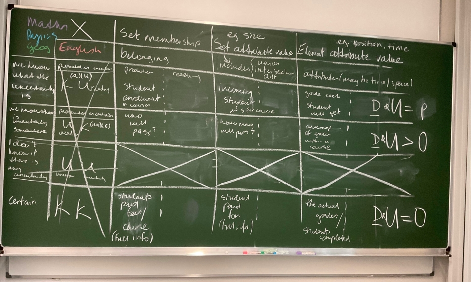
Overall, the discussion of the characteristics of set data $D$ and the types of uncertainty $U$ led us to a conceptual framework of uncertainty in set visualization. In terms of $D$, the framework distinguishes: set membership, set attributes, and element attributes. Related to $U$, we use the different plausible types of (un)certainty: certainty ($U=0$), uncertainty as a binary fact ($U>0$), and uncertainty as quantifiable measure ($U=p$). We captured the framework in a table whose columns and rows respectively represent $D$ and $U$, as shown in fig. 7.

Based on this conceptual framework, we then systematically discussed possible visualization designs to illustrate examples and highlight challenges of integrating uncertainty in set visualizations. Three subgroups were formed, each working on a selected data characteristic (i.e., table column). As a baseline, each subgroup used the simple case of a visual representation with zero uncertainty ($U=0$). The group that dealt with set membership worked with bi-partite node-link and matrix representations, which were gradually expanded to include unknown uncertainty ($U>0$) and known uncertainty ($U=p$) by varying the visual encoding of links and matrix cells as indicated in fig. 8.

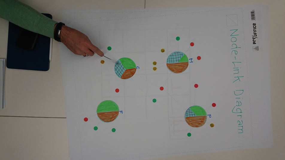
Set attributes turned out to be particularly challenging to visualize when uncertainty is involved. The reason for this is that derived data attributes depend by definition on other data characteristics, which also can include varying levels of uncertainty. For example, set size depends on set memberships. Leaving this particular challenge for future work, the subgroup designed and discussed visual representations where set attributes do not depend on other factors. They came up with node-link-style representations as shown in fig. 9. Sets are represented as bigger nodes being linked to their belonging set elements, which are depicted as smaller nodes. The set attributes are shown as pie charts within the bigger nodes, where color hue indicates certain attribute values and hatching marks uncertain set elements. The same encoding is applied to the attributes of the individual set elements on the smaller nodes.

Finally, one subgroup worked on visualizing uncertain element attributes. Their focus was not so much on coming up with new designs, but to review the existing knowledge about general uncertainty visualization. For example, cartography has a long history in working with uncertain data, but also the visualization community studied this topic in detail. Particularly, the works by Alan MacEachren et al. [5, 6], Kristin Potter et al. [7, 8, 2], Amit Jena et al. [4], and Theresia Gschwandtner et al. [3] offer profound insight into how uncertain data values can be encoded visually, and to what degree humans can interpret and understand the depicted information. With these general considerations, the table of the developed conceptual framework could be filled completely. Based on the intense and productive discussions centered on the conceptual framework for set visualization and uncertainty, we drafted an outline for a journal article that will summarize key results of the research conducted at the Dagstuhl-Seminar. Our planned article will also include a synthesis of recommendations to be considered when designing visualizations for uncertain set data and an outline of future research directions.

This working group consisted of (in alphabetical order) Michael Behrisch, Susanne Bleisch, Sarah Fabrikant, Eva Mayr, Silvia Miksch, Helen Purchase, and Christian Tominski (see fig. 10). Helen Purchase headed the group. Christian Tominski drafted this report. All members of the team contributed significantly to the discussions, provided feedback and edited this report, and will be co-authors of the planned journal article.

References

- [1] Munzner, T. (2014). Visualization Analysis & Design. Boca Raton: CRC Press.
- [2] Padilla, L. and Kay, M. and Hullman, J. (2021). Uncertainty Visualization in Wiley StatsRef: Statistics Reference Online. Eds. N. Balakrishnan and T. Colton and B. Everitt and W. Piegorsch and F. Ruggeri and J.L. Teugels, Wiley. doi:10.1002/9781118445112.
- [3] Alsallakh, Bilal and Micallef, Luana and Aigner, Wolfgang and Hauser, Helwig and Miksch, Silvia and Rodgers, Peter (2016). The State-of-the-Art of Set Visualization. Computer Graphics Forum, 35(1):234–260. doi:10.1111/cgf.12722.
- [4] Steven Chaplick and Takayuki Itoh and Giuseppe Liotta and Kwan-Liu Ma and Ignaz Rutter (2020). Trends and Perspectives in Graph Drawing and Network Visualization, NII Shonan Meeting Report 171. https://shonan.nii.ac.jp/docs/342e2e86373d4783ae00063ddd67e8b35b9d75d5.pdf.
- [5] MacEachren, Alan M. and Robinson, Anthony and Hopper, Susan and Gardner, Steven and Murray, Robert and Gahegan, Mark and Hetzler, Elisabeth (2005). Visualizing Geospatial Information Uncertainty: What We Know and What We Need to Know. Cartography and Geographic Information Science, 32(3):139–160. doi:10.1559/1523040054738936.
- [6] Görtler, Jochen and Schulz, Christoph and Weiskopf, Daniel and Deussen, Oliver (2018). Bubble Treemaps for Uncertainty Visualization. IEEE Transactions on Visualization and Computer Graphics, 24(1):719–728. doi:10.1109/TVCG.2017.2743959.
- [7] Sondag, Max and Meulemans, Wouter and Schulz, Christoph and Verbeek, Kevin and Weiskopf, Daniel and Speckmann, Bettina (2020). Uncertainty Treemaps. 2020 IEEE Pacific Visualization Symposium (PacificVis), 111–120. IEEE.
- [8] Xu, Kai and Salisu, Saminu and Nguyen, Phong H. and Walker, Rick and Wong, B. L. William and Wagstaff, Adrian and Phillips, Graham and Biggs, Mike and Potel, Mike (2020). TimeSets: Temporal Sensemaking in Intelligence Analysis. IEEE Computer Graphics and Applications, 40(3):83–93. doi:10.1109/MCG.2020.2981855.
- [9] Zhu, Lifeng and Xia, Weiwei and Liu, Jia and Song, Aiguo (2018). Visualizing fuzzy sets using opacity-varying freeform diagrams. Information Visualization, 17(2):146–160.doi:10.1177/1473871617698517.
- [10] Vullings, L. A. E. and Blok, C. A. and Wessels, C. G. A. M. and Bulens, J. D. (2013). Dealing with the uncertainty of having incomplete sources of geo-information in spatial planning. In Applied spatial analysis and policy, 6(1):25–45. Springer.
- [11] Vehlow, Corinna and Reinhardt, Thomas and Weiskopf, Daniel (2013). Visualizing Fuzzy Overlapping Communities in Networks. IEEE Transactions on Visualization and Computer Graphics, 19(12):2486–2495. doi:10.1109/TVCG.2013.232.
2 Table of Contents
3 Overview of Talks
3.1 (Invited) Drawing Euler Diagrams with Closed Curves
Daniel Archambault (Swansea University, GB)
License: ![]() Creative Commons BY 4.0 International license © Daniel Archambault
Creative Commons BY 4.0 International license © Daniel Archambault
Joint work of: Paolo Simonetto, Daniel Archambault, Carlos Scheidegger, David Auber
One of the typical methods for visualising sets is through Euler diagrams represented as closed curves. In this talk, I recap some work on force-directed drawings of Euler diagrams and the scalability of such methods. In particular, I speak of force-directed methods for drawing Euler diagrams and methods for refining them given a drawing. I conclude with some open problems that involve representing uncertainty in this representation.
3.2 (Invited) Algorithmic Perspectives on Uncertainty and Set Visualization
Wouter Meulemans (TU Eindhoven, NL)
License: ![]() Creative Commons BY 4.0 International license © Wouter Meulemans
Creative Commons BY 4.0 International license © Wouter Meulemans
Treemaps are a common way to visualize hierarchical numeric data (file systems, census data, economic data). However, in many cases, the numeric values have associated uncertainty: arising for example from the data-collection process or from data transformations like aggregation over time. I will discuss a method [1] for creating treemaps that show both the data itself and the uncertainty, while maintaining the partitioning nature of treemaps. Then, I continue briefly to consider an alternative perspective: to artificially induce uncertainty to improve visual structure. Specifically, we will look at using spatial deformation to schematize set visualization [2] and relate this to research in algorithmic imprecision.
- [1] M. Sondag, W. Meulemans, C. Schulz, K. Verbeek, D. Weiskopf, and B. Speckmann. Uncertainty treemaps. In Proceedings of the 2020 IEEE Pacific Visualization Symposium, pages 111–120, 2020.
- [2] M. A. Bekos, D. J. C. Dekker, F. Frank, W. Meulemans, P. Rodgers, A. Schulz, and S. Wessel. Computing Schematic Layouts for Spatial Hypergraphs on Concentric Circles and Grids. Computer Graphics Forum, 41(6):316–335, 2022.
3.3 (Invited) Visualizing Hypergraphs: With Connections to Uncertainty Visualization
Bei Wang Phillips (University of Utah – Salt Lake City, US)
License: ![]() Creative Commons BY 4.0 International license © Bei Wang Phillips
Creative Commons BY 4.0 International license © Bei Wang Phillips
Joint work of: Bei Wang Phillips, Youjia Zhou, Archit Rathore, Emilie Purvine, Samir Chowdhury, Tom Needham, Ethan Semrad
- [1] MacEachren, Alan M. and Robinson, Anthony and Hopper, Susan and Gardner, Steven and Murray, Robert and Gahegan, Mark and Hetzler, Elisabeth (2005). Visualizing Geospatial Information Uncertainty: What We Know and What We Need to Know. Cartography and Geographic Information Science, 32(3):139–160. doi:10.1559/1523040054738936.
- [2] Alan M. MacEachren, Robert E. Roth, James O’Brien, Bonan Li, Derek Swingley, Mark Gahegan: Visual Semiotics & Uncertainty Visualization: An Empirical Study. IEEE Trans. Vis. Comput. Graph. 18(12): 2496-2505 (2012).
3.7 (Contributed) Visual Encodings of Temporal Uncertainty: A Comparative User Study
Silvia Miksch (TU Wien, AT)
License: ![]() Creative Commons BY 4.0 International license © Silvia Miksch
Creative Commons BY 4.0 International license © Silvia Miksch
Joint work of: Theresia Gschwandtner, Markus Bögl, Paolo Federico, Silvia Miksch
- [1] T. Herrmann. Storyline visualizations for scientific collaboration graphs. Master’s thesis, Institut für Informatik, Universität Würzburg, 2022. URL: https://www1.pub.informatik.uni-wuerzburg.de/pub/theses/2022-herrmann-masterarbeit.pdf.
- [2] T. C. van Dijk, M. Fink, N. Fischer, F. Lipp, P. Markfelder, A. Ravsky, S. Suri, and A. Wolff. Block crossings in storyline visualizations. J. Graph Alg. Appl., 21(5):873–913, 2017. doi:10.7155/jgaa.00443.
4 Working groups
4.1 StorySets
Annika Bonerath (Universität Bonn, DE), Stephen G. Kobourov (University of Arizona – Tucson, US), Wouter Meulemans (TU Eindhoven, NL), Martin Nöllenburg (TU Wien, AT), Markus Wallinger (TU Wien, AT), and Alexander Wolff (Universität Würzburg, DE)
License: ![]() Creative Commons BY 4.0 International license © Annika Bonerath, Stephen G. Kobourov, Wouter Meulemans, Martin Nöllenburg, Markus Wallinger, and Alexander Wolff
Creative Commons BY 4.0 International license © Annika Bonerath, Stephen G. Kobourov, Wouter Meulemans, Martin Nöllenburg, Markus Wallinger, and Alexander Wolff
Problem Definition
Roughly speaking, there are two types of set systems: abstract and spatial. In a spatial set system, each element has a fixed, spatial location. Visualizations of spatial set systems usually use connected regions of the plane in order to visualize the sets: elements are points in the plane, and a set consists of exactly those elements that lie inside the region. Examples for such visualizations are Bubble Sets [4], GMap [8], or MapSets [6]. LineSets [1] connect the elements of a set by a path. LineSets are generalized by Kelp diagrams [5], which connect the elements of a set by a sparse spanning graph. In order to avoid intersections, ClusterSets [9] allow disconnected regions to visualize sets. Examples for visualizations of abstract set systems are Venn diagrams, Euler diagrams [7], linear diagrams [11], matrices, etc. The survey by Alsallakh et al. [2] gives an extensive overview over methods for set visualization.
A fuzzy set system consists of a finite universe of elements and a finite collection of fuzzy sets. A fuzzy set in is described by a membership function that expresses the certainty of element being in set . For example, if , then is certainly contained in , and if , then is certainly not contained in . We assume that membership functions are independent of each other.
During the seminar, we investigated various ways to graphically represent fuzzy set systems. We focussed on visualizing (uncertain) set membership per element and (uncertain) set containment. Specifically, if for every , then we say that is uncertainly contained in , and we would like this relationship to be graphically represented as well. Note, however, that uncertain containment does not guarantee containment.
Exploring the Design Space
During the seminar, we first tried to extend visualizations for spatial set systems to the fuzzy case. We considered representing elements as unit-sized disks instead of points; see Figure 4b for an adaption of Euler diagrams and Figure 4c for an adaption of LineSets. In order to indicate how certain the membership of an element in a set is we used the element’s distance to the set boundary or partial containment of the element in the set’s region. The latter type of representation may be somewhat more intuitive; see Figure 4b and Figure 4c.
Second, we looked at an adaptation of linear diagrams [11]; see Figure 4d. Each set is a row in this matrix, and each element is a column. The certainty of the membership is illustrated by the line width. A disadvantage of this visualization is that it is difficult to recognize (uncertain) set containment.
Third, we explored a style in which sets are represented as curves and elements as axes that are intersected by the set curves. For example, in a star plot [3], axes are radials emanating from a common center and a set (or, by duality, an element) is represented by a polygon whose vertices lie on these axes. The distance of a polygon vertex from the center of the diagram expresses the value of some parameter. For visualizing fuzzy set systems, we introduced an axis for each element and chose as parameter to be displayed on its axis the membership certainty of in ; see Figure 4e. This visualization easily encodes uncertain set containment via polygon containment.
However, this principle can be applied more generally, using ideas found in, e.g, Sankey diagrams [12] and storyline visualizations [10, 13]. Specifically, we explored a novel design that combines storylines and set visualization. For this design, we assume that membership certainties are grouped into a few certainty groups, e.g., by rounding. Now, we can partition the axis of an element according to the number of sets per uncertainty group. We represent every element by a stack of boxes such that each box represents one certainty group. In this representation, the width of a box encodes the certainty and the height of a box encoding the number of sets that contain the element with the given certainty. The box for the highest certainty group is anchored at the top and the others are placed underneath, ordered by their certainty value. We call this visualization StorySets; see Figure 4f. With this visualization (uncertain) set containment is encoded as follows: if the curve of a set is always below the curve of another set , then the is uncertainly contained in . We consider StorySets a promising approach for the visualization of fuzzy set systems and, hence, focused on StorySets for the remainder of the seminar.
During the discussion, we considered several variants of StorySets, some needing only small adjustments (e.g., a different choice of symbols; see Figure 5a); others posing new algorithmic problems (e.g., compactness; see Figure 5b). In the following, we discuss three of these variants.
Compactness
We can vertically compact a StorySet representation by not showing every set curve for the whole time, that is, over the complete horizontal extent of the diagram. Instead, we allow each set curve to start immediately before its respective first element in the given element order and to end right after its respective last element; see Figure 5b.
Also, it is possible to horizontally compact the design by considering “non-linear” storylines. To this end, we can stack an element above an element if (it is certain that) there is no set that contains both and ; see Figure 5b.
Fixed heights per certainty box
Due to the varying heights of the certainty boxes throughout the elements, it might be difficult to perceive whether a curve changes the certainty level between two elements or not. Hence, we considered the variant that we have a fixed height per certainty group defined by the maximal number of sets in which an element is contained; see Figure 5c.
Circular arrangement
We want to mention that the optimization for horizontal arrangement of elements can be easily adapted to a circular arrangement of elements. Here, one only needs to take care about the additional cyclic constraints between the last and the first element.
Algorithmic Considerations
The designs discussed in the last section give rise to several optimization problems. In the case of star plots, linear diagrams or StorySets, the order of the elements is very important. Ideally, we would like to place elements with similar fuzzy set memberships next to each other resulting in more homogeneous curves and polygons. Since each element can be seen as an -dimensional vector in a matrix, we can define a distance metric between them and model this as an ordering problem. Depending on the visualization design, computing the linear arrangement or profile of the matrix, or modelling it as a traveling salesperson problem, could be used to tackle this optimization problem.
Specifically for StorySets, it seems natural to consider the following optimization goals: (i) minimize the number of curve crossings, (ii) minimize the number of level changes over all curves, and (iii) keep the drawing compact, that is, minimize width and/or height. In order to achieve these design goals, we want to find a horizontal order of the elements and a vertical order of the curves that respects the certainty groups of each element. Note that goals (i) and (ii) are very similar to what standard storylines aim to optimize [10].
We worked on a pipeline that alternates between the optimization of the horizontal order of the elements and the vertical order of the curves per certainty box and per element. First, we fix the vertical order of curves per element such that the certainty groups are respected. Second, we compute the number of crossings between every pair of elements. Third, we introduce an auxiliary complete graph where each vertex corresponds to an element and each edge is weighted with the number of crossing curves if the two elements are consecutive in the horizontal order. Then, we solve the traveling salesperson problem on this graph. This leads to a new horizontal order of the elements. Now, if we can further improve the vertical order of the curves per element, we return to the first step. Otherwise, the algorithm terminates.
Outlook
We plan to provide an framework with several algorithms for computing various versions of StorySets. We want to evaluate our approach using real-world data. Such real-world data could be, for example, a set of tweets combined with a topic analysis. Each topic then corresponds to a set and the certainty with which a tweet belongs to a topic reflects its uncertain membership in that set.
- [1] B. Alper, N. Henry Riche, G. Ramos, and M. Czerwinski. Design study of LineSets, a novel set visualization technique. IEEE Trans. Vis. Comput. Graphics, 17(12):2259–2267, 2011. doi:10.1109/TVCG.2011.186.
- [2] B. Alsallakh, L. Micallef, W. Aigner, H. Hauser, S. Miksch, and P. J. Rodgers. The state-of-the-art of set visualization. Comput. Graphics Forum, 35(1):234–260, 2016. doi:10.1111/cgf.12722.
- [3] J. Chambers, W. Cleveland, B. Kleiner, and P. Tukey. Graphical Methods for Data Analysis. Wadsworth, 1983.
- [4] C. Collins, G. Penn, and S. Carpendale. Bubble Sets: Revealing set relations with isocontours over existing visualizations. IEEE Trans. Vis. Comput. Graphics, 15(6):1009–1016, 2009. doi:10.1109/TVCG.2009.122.
- [5] K. Dinkla, M. van Kreveld, B. Speckmann, and M. A. Westenberg. Kelp diagrams: Point set membership visualization. Comput. Graphics Forum, 31(3):875–884, 2012. doi:10.1111/j.1467-8659.2012.03080.x.
- [6] A. Efrat, Y. Hu, S. G. Kobourov, and S. Pupyrev. MapSets: Visualizing embedded and clustered graphs. J. Graph Algorithms Appl., 19(2):571–593, 2015. doi:10.7155/jgaa.00364.
- [7] J. Flower, A. Fish, and J. Howse. Euler diagram generation. J. Vis. Lang. Comput., 19(6):675–694, 2008. doi:10.1016/j.jvlc.2008.01.004.
- [8] E. R. Gansner, Y. Hu, and S. G. Kobourov. GMap: Visualizing graphs and clusters as maps. In Proc. Pacific Vis. Symp. (PacificVis), pages 201–208. IEEE, 2010. doi:10.1109/PACIFICVIS.2010.5429590.
- [9] J. Geiger, S. Cornelsen, J.-H. Haunert, P. Kindermann, T. Mchedlidze, M. Nöllenburg, Y. Okamoto, and A. Wolff. ClusterSets: Optimizing planar clusters in categorical point data. Comput. Graphics Forum, 40(3):471–481, 2021. doi:10.1111/cgf.14322.
- [10] I. Kostitsyna, M. Nöllenburg, V. Polishchuk, A. Schulz, and D. Strash. On minimizing crossings in storyline visualizations. In E. D. Giacomo and A. Lubiw, editors, Proc. 23rd Int. Symp. Graph Drawing Network Vis. (GD’15), volume 9411 of LNCS, pages 192–198. Springer, 2015. URL: https://arxiv.org/abs/1509.00442, doi:10.1007/978-3-319-27261-0_16.
- [11] P. J. Rodgers, G. Stapleton, and P. Chapman. Visualizing sets with linear diagrams. ACM Trans. Comput. Hum. Interact., 22(6):27:1–27:39, 2015. doi:10.1145/2810012.
- [12] M. H. P. R. Sankey. Introductory note on the thermal efficiency of steam-engines. In Minutes of Proceedings of the Institution of Civil Engineers, volume 134, pages 278–283, 1898.
- [13] T. C. van Dijk, M. Fink, N. Fischer, F. Lipp, P. Markfelder, A. Ravsky, S. Suri, and A. Wolff. Block crossings in storyline visualizations. J. Graph Alg. Appl., 21(5):873–913, 2017. doi:10.7155/jgaa.00443.
4.2 Simplification of Set Systems to Draw Nice Euler Diagrams
Peter Rodgers (University of Kent – Canterbury, GB), Daniel Archambault (Swansea University, GB), Jan-Henrik Haunert (Universität Bonn, DE), and Bei Wang Phillips (University of Utah – Salt Lake City, US)
License: ![]() Creative Commons BY 4.0 International license © Peter Rodgers, Daniel Archambault, Jan-Henrik Haunert, and Bei Wang Phillips
Creative Commons BY 4.0 International license © Peter Rodgers, Daniel Archambault, Jan-Henrik Haunert, and Bei Wang Phillips
Motivation and general idea
Euler diagrams are frequently used to visualize set systems. They represent each set as a region that is bounded by a closed curve. An area in an Euler diagram where multiple regions overlap indicates the existence of set elements that are contained in the corresponding sets and in no other set. An advantage of Euler diagrams is that they are intuitive to understand. However, they can become cluttered even for medium-sized set systems. When requiring the regions to be contiguous, it may even be the case that for a given set system no Euler diagram exists. We aim to mitigate these weaknesses of Euler diagrams by developing algorithms for the simplification of set systems. Given a set system as input, our goal is to compute a simplified but still similar version of it that can be drawn nicely as an Euler diagram. In this report we introduce a measure of dissimilarity between a set system and a simplified version of it (i.e., a distance) and state the criteria a set system needs to fulfill such that it can be drawn nicely. Based on this we sketch an optimization approach as well as a greedy heuristic. While a lot of previous work on the automatic generation of Euler diagrams exists [1, 2, 3, 4, 5, 6, 7, 8], we hope that with our simplification algorithms we will be able to extend the applicability of Euler diagrams to much larger and more complex set systems.
Preliminaries
Formally we consider a set system as a bipartite graph ; see Fig. 6(a). Every node represents an element and every node a set. Every edge indicates that element is a member of set . The set of all elements is partitioned into zones such that, if two elements are members of exactly the same sets in , then and are in the same zone. A zone is labeled with the sets in that have its elements as members. With we refer to the set of labels of a zone . Our algorithms operate on a graph that contains a node for each zone and an edge between every two zones that share at least one label; see Fig. 6(b). In particular, our optimization algorithm computes a subgraph of such that, in a next processing step, we can compute an Euler diagram whose dual graph is . Accordingly, we call the super dual graph. Figure 6(c) shows a subgraph of the super dual graph in Fig. 6(b). An Euler diagram that has as its dual graph is shown in Fig. 6(d).
Distance measure
Since we aim for a set system that is similar to the input set system , we need to quantify the loss of information resulting from the reduction of the super dual graph to the dual graph of the Euler diagram. We do this by computing an optimal assignment that maps every zone that is not selected for to a selected zone or to the empty set . Each assignment of a zone to a zone is interpreted such that the elements in are removed from every set in and inserted into every set in . If is asssigned to , then the elements in are removed from every set in but not inserted into any set. For every removal of an element from a set and every insertion of an element into a set we charge a cost and , respectively. The transport distance between the two set systems represented by and is the minimum total cost over all possible assignments.
Optimization problem
We are now ready to define the task of simplifying a set system as an optimization problem.
SetSystemSimplification:
Given the super dual graph of a set system , find a subgraph of
such that
-
(1)
is planar,
(2)
for every set , the subgraph of induced by the set of zones labeled with is connected or empty, and
(3)
the transport distance between the set systems represented by and is minimized.
Optionally, to keep the visual complexity of the output Euler diagram low, we could require to select at most a prescribed number of zones. Furthermore, to avoid concurrencies in the output Euler diagram (which is one of the criteria for well-formed Euler diagrams), we could discard all edges of whose incident zones differ by more than one label. To compute an optimal solution, we consider Integer Linear Programming, but also local search seems promising.
Greedy heuristic
Our greedy heuristic takes the super dual graph as input and iterates until a certain set of conditions is reached. In each iteration, we select two intersecting sets and and merge them to one. We update to reflect this change. In principle, we could choose and arbitrarily (as long as they intersect). However, to get closer to a sufficiently simplified version of the set system, we prioritize the different options as follow:
A merge of two sets and has highest priority if it destroys a subgraph of that is a Kuratowski subdivision, i.e., a subdivision of one of the two non-planar graphs or . This is because it will bring us closer to a planar graph, which is strictly required for drawing the Euler diagram.
Our second priority is to choose a merge if it destroys a concurrency.
If multiple merges are equally good according to the first two criteria, we choose the merge based on a measure of (dis-)similarity. In particular, we consider choosing the merge that yields the set system at minimum transport distance from the current set system, but it would also be reasonable to merge the two sets with maximum Jaccard similarity.
Final remarks
We consider the optimization approach and the greedy heuristic as two complementary approaches, which we plan to implement and compare in experiments. Concerning the rendering of an Euler diagram based on its dual graph our hope is that we can re-use existing methods and software. A crucial question that needs further discussions, however, is how the uncertainties introduced with our simplification methods can be visualized.
- [1] Jean Flower and John Howse. Generating Euler diagrams. In Proc. 2nd International Conference on Diagrammatic Representation and Inference (Diagrams 2002), pages 61–75, 2002.
- [2] Peter Rodgers, Leishi Zhang, and Andrew Fish. General Euler diagram generation. In Proc. 5th International Conference on Diagrammatic Representation and Inference (Diagrams 2008), pages 13–27, 2008.
- [3] Peter Rottmann, Markus Wallinger, Annika Bonerath, Sven Gedicke, Martin Nöllenburg, and Jan-Henrik Haunert. MosaicSets: Embedding set systems into grid graphs. IEEE Transactions on Visualisation and Computer Graphics, 29(1):875–885, 2023.
- [4] Paolo Simonetto, Daniel Archambault, and Carlos Scheidegger. A simple approach for boundary improvement of Euler diagrams. IEEE Transactions on Visualization and Computer Graphics, 22(1):678–687, 2016.
- [5] Paolo Simonetto and David Auber. Visualise undrawable Euler diagrams. In Proc. 12th International Conference Information Visualisation, pages 594–599, 2008.
- [6] Paolo Simonetto and David Auber. An heuristic for the construction of intersection graphs. In Proc. 13th International Conference Information Visualisation, pages 673–678, 2009.
- [7] Paolo Simonetto, David Auber, and Daniel Archambault. Fully automatic visualisation of overlapping sets. In Proc. 11th Eurographics / IEEE – VGTC Symposium on Visualization (EuroVis’09), pages 967–974, 2009.
- [8] Youjia Zhou, Archit Rathore, Emilie Purvine, and Bei Wang. Topological simplifications of hypergraphs. IEEE Transactions on Visualization and Computer Graphics, 2022.
4.3 Types of Uncertainty in Set Visualization
Christian Tominski (Universität Rostock, DE), Michael Behrisch (Utrecht University, NL), Susanne Bleisch (FH Nordwestschweiz – Muttenz, CH), Sara Irina Fabrikant (Universität Zürich, CH), Eva Mayr (Donau-Universität Krems, AT), Silvia Miksch (TU Wien, AT), and Helen C. Purchase (Monash University – Clayton, AU)
License: ![]() Creative Commons BY 4.0 International license © Christian Tominski, Michael Behrisch, Susanne Bleisch, Sara Irina Fabrikant, Eva Mayr, Silvia Miksch, and Helen C. Purchase
Creative Commons BY 4.0 International license © Christian Tominski, Michael Behrisch, Susanne Bleisch, Sara Irina Fabrikant, Eva Mayr, Silvia Miksch, and Helen C. Purchase
- [1] Bilal Alsallakh, Luana Micallef, Wolfgang Aigner, Helwig Hauser, Silvia Miksch, and Peter J. Rodgers. The State-of-the-Art of Set Visualization. Comput. Graph. Forum, 35(1):234–260, 2016. doi:10.1111/cgf.12722.
- [2] Georges-Pierre Bonneau, Hans-Christian Hege, Chris R. Johnson, Manuel M. Oliveira, Kristin Potter, Penny Rheingans, and Thomas Schultz. Overview and State-of-the-Art of Uncertainty Visualization. In Charles D. Hansen, Min Chen, Christopher R. Johnson, Arie E. Kaufman, and Hans Hagen, editors, Scientific Visualization, Mathematics and Visualization, pages 3–27. Springer, 2014. doi:10.1007/978-1-4471-6497-5\_1.
- [3] Theresia Gschwandtner, Markus Bögl, Paolo Federico, and Silvia Miksch. Visual Encodings of Temporal Uncertainty: A Comparative User Study. IEEE Trans. Vis. Comput. Graph., 22(1):539–548, 2016. doi:10.1109/TVCG.2015.2467752.
- [4] Amit Jena, Ulrich Engelke, Tim Dwyer, Venkatesh Raiamanickam, and Cécile Paris. Uncertainty Visualisation: An Interactive Visual Survey. In 2020 IEEE Pacific Visualization Symposium, PacificVis 2020, Tianjin, China, June 3-5, 2020, pages 201–205. IEEE, 2020. doi:10.1109/PacificVis48177.2020.1014.
- [5] Alan M. MacEachren, Anthony Robinson, Susan Hopper, Steven Gardner, Robert Murray, Mark Gahegan, and Elisabeth Hetzler. Visualizing Geospatial Information Uncertainty: What We Know and What We Need to Know. Cartography and Geographic Information Science, 32(3):139–160, 2005. doi:10.1559/1523040054738936.
- [6] Alan M. MacEachren, Robert E. Roth, James O’Brien, Bonan Li, Derek Swingley, and Mark Gahegan. Visual Semiotics & Uncertainty Visualization: An Empirical Study. IEEE Trans. Vis. Comput. Graph., 18(12):2496–2505, 2012. doi:10.1109/TVCG.2012.279.
- [7] Kristin Potter. The Visualization of Uncertainty. PhD thesis, University of Utah, USA, 2010.
- [8] Kristin Potter, Joe Kniss, Richard F. Riesenfeld, and Chris R. Johnson. Visualizing Summary Statistics and Uncertainty. Comput. Graph. Forum, 29(3):823–832, 2010. doi:10.1111/j.1467-8659.2009.01677.x.
4.4 Set Size Visualization with Dependent and Independent Uncertainties
Nathan Van Beusekom (TU Eindhoven, NL), Steven Chaplick (Maastricht University, NL), Amy Griffin (RMIT University – Melbourne, AU), Martin Krzywinski (BC Cancer Research Centre – Vancouver, CA), Marc van Kreveld (Utrecht University, NL), and Hsiang-Yun Wu (FH – St. Pölten , AT)
License: ![]() Creative Commons BY 4.0 International license © Nathan Van Beusekom, Steven Chaplick, Amy Griffin, Martin Krzywinski, Marc van Kreveld, and Hsiang-Yun Wu
Creative Commons BY 4.0 International license © Nathan Van Beusekom, Steven Chaplick, Amy Griffin, Martin Krzywinski, Marc van Kreveld, and Hsiang-Yun Wu
Problem Setting
We discuss the visualization of set sizes and their uncertainties. We distinguish between independent and dependent uncertainty in set sizes, where the latter refers to elements that are certainly present, but it is unknown to which set they belong, among two (or more) possibilities. We present three options to visualize sets sizes and their uncertainties. For each, we discuss when to use them and what their advantages and disadvantages are.
Related Work
Sets are models that have been used in data management and analysis to capture collection relationships of elements. In addition, uncertainty information provides more context regarding the reliability of the underlying data sets. Classical uncertainty visualizations cover not only visual language design [6], but also its corresponding visual efficiency [4]. Although several set visualization algorithms have been proposed [1], integrating uncertainty into these approaches is still in its infancy.
Visualizing uncertainty in sets is related to the problem of visualizing Fuzzy Sets [10], where membership is a value between 0 and 1. Disk diagrams [8] interactively visualize fuzzy sets, and show the membership distribution of the elements with one disk per set.
Some visualization approaches for independent set uncertainty have been proposed. For example, Uncertainty Treemaps [9], introduced nested hatched lines to show the independent set uncertainty for treemaps across hierarchies. Another example of visualizing independent set size uncertainty for hierarchical data is Bubble Treemaps [3], which use squiggly lines to indicate uncertainty. UpSet [5] lists essential combinations of sets, especially their intersections, and aggregates of intersections. Showing independent and dependent set size uncertainties has not yet been fully investigated to the best of our knowledge.
Visual Design for Set Data with Dependent and Independent Uncertainties
The visualization of set sizes rather than sets with their elements allows us to use part of the available space for visualizing the set size uncertainty, since we do not need to show the elements in the sets themselves. Visualization of set size is best done by using a visual variable related to size, e.g., area or length. This holds true for the uncertainty in the set size as well. Studies show that people can intuitively understand uncertainties when they are expressed as frequencies [2]. Directly depicting both set sizes and set size uncertainties with size makes comparisons between sets easier by offloading the cognitive effort of mental arithmetic onto vision [7].
There are various scenarios where understanding the size of a set is more important than understanding set membership. Some of these scenarios have a geographic component while others do not. We therefore consider different visualization options.
A visualization of set sizes and their uncertainties should be able to show answers to the following questions:
1.
For each set, what is its minimum and maximum size, and how much uncertainty is there in the size?
2.
What sets can be the largest sets?
3.
Between which sets does a large dependent size uncertainty exist?
If the visualization shows the spatial location of the sets as well, we additionally want it to be able to answer the following questions:
Where are the smaller or larger regions located?
Where are the regions with more uncertainty located?
Discussion
We describe several types of set size uncertainty visualization and some of their affordances and challenges next. To illustrate a basic visualization of such a data set, we use proportional disks drawn in a node-link style (Fig. 2A) where dependencies are indicated with edges/connections between disks.
- Topic 1.
Sets are commonly represented as disks with proportional size, such as in Euler diagrams. We use a simple visualization to explain the concepts of dependent and independent uncertainty (Fig. 2A). The certain set sizes are represented as gray disks, independent uncertainties as blue disks attached to the gray disks, and dependent uncertainties as pink disks, with lines connecting them to the corresponding gray disks.
Though this visualization may introduce some clutter, it allows for showing more dependencies than the other visualizations, by efficiently placing the gray disks in the plane.
Furthermore, it naturally allows for showing dependency between more than two sets, by simply adding extra lines to the additional dependent gray disks.
- Topic 2.
Bar charts (Fig. 2B) are a simple and effective way to show sizes of sets. It is intuitive to stack uncertain set size bars on top of the bars that show certain sizes. This idea implies that the certain parts show the minimum set size, and we must adopt an additive view of set size. The maximum set size is implied by the length of all bar parts considered together.
Every set has three types of bars that should be distinguishable: a bar for the certain part, a part for the independently uncertain part, and zero or more bars that represent sizes of dependent uncertainties. In case of pairwise uncertainties, these bars always come in pairs, and we use a line connecting the two bars that are interdependent.
In the visualization, we have the choice of ordering the sets (bars) from left to right in a convenient way. We also have the choice of ordering the dependently uncertain components vertically. These choices influence how complex the connecting lines get, for example, whether they intersect and how long they are.
We think that this type of visualization is the most clear, but it is limited to at most a few dozen sets and it cannot show geographic patterns.
- Topic 3.
In a second visualization type, we examined rectangular subdivisions like rectangular cartograms and treemaps (Fig. 2D). They allow the visualization to distort the spatial location of the sets and use the available two-dimensional space more efficiently than either bar charts or the reservoir maps when there are many sets. Each set is shown by a rectangle whose size represents the size of the set. If the set represents a geographic region like a country, then these visualizations attempt to maintain adjacencies and relative orientations.
On the border between two rectangles we can show the dependent uncertainties that may exist between adjacent locations. For example, a gas station close to the border between two countries may have clientele from both countries. We may know the total sales of petrol, but not how much exhaust will be caused by this petrol in each of the two countries. Such dependent size uncertainty is shown by a region that overlaps the border and extends on both sides of it.
Independent size uncertainty, which includes uncertainty that is definitely attributable to a specific set (in this case, a location), is shown at the edge of each rectangle, but how a reader will interpret any visualization that does this is unclear. Another issue is that dependent uncertainties between non-adjacent regions are difficult show.
- Topic 4.
We examine a new style of visualization that we call Reservoir Maps (Fig. 2C). They are suitable when a (geographic) map has regions that represent the sets. They are similar to the visualization using rectangular subdivisions, but here we show regions as they are, and use proportional symbols or enumeration symbols to show the set sizes and their uncertainties. The effect is that we use less space for the visualization of the set size variable, but provide a stronger connection to the actual region (in case it needs to be be easily recognizable).
Because the set size corresponding to a region is now symbolized, we can show the certain and independently uncertain parts better inside the region than with rectangular subdivisions. The dependent size uncertainties are again shown in a way that overlaps the border defining the dependency.
The symbol type used for the certain sizes, the independently uncertain sizes, and the dependently uncertain sizes should be the same. We could use a proportional symbol like a disk for each set size component, or an enumeration symbol like small squares. Color can be used to visualize what size is certain and what size is uncertain.
An issue is that dependent uncertainties between non-adjacent regions are difficult show, and it may be challenging to scale symbol sizes for small regions that have large set sizes because this visualization does not distort space.
These visualization types are static. With interaction, many additional options exist for focus and details on demand.
Acknowledgment.
The topic was proposed by Wouter Meulemans.
- [1] Bilal Alsallakh, Luana Micallef, Wolfgang Aigner, Helwig Hauser, Silvia Miksch, and Peter Rodgers. The state-of-the-art of set visualization. Computer Graphics Forum, 35(1):234 – 260, 2016.
- [2] Gerd Gigerenzer. The psychology of good judgment: Frequency formats and simple algorithms. Medical Decision Making, 16(3):273–280, 1996. PMID: 8818126.
- [3] Jochen Görtler, Christoph Schulz, Daniel Weiskopf, and Oliver Deussen. Bubble treemaps for uncertainty visualization. IEEE transactions on visualization and computer graphics, 24(1):719–728, 2017.
- [4] Jessica Hullman, Xiaoli Qiao, Michael Correll, Alex Kale, and Matthew Kay. In pursuit of error: A survey of uncertainty visualization evaluation. IEEE Transactions on Visualization and Computer Graphics, 25(1):903–913, 2019.
- [5] Alexander Lex, Nils Gehlenborg, Hendrik Strobelt, Romain Vuillemot, and Hanspeter Pfister. Upset: Visualization of intersecting sets. IEEE Transactions on Visualization and Computer Graphics, 20(12):1983–1992, 2014.
- [6] Alan M. MacEachren, Robert E. Roth, James O’Brien, Bonan Li, Derek Swingley, and Mark Gahegan. Visual semiotics & uncertainty visualization: An empirical study. IEEE Transactions on Visualization and Computer Graphics, 18(12):2496–2505, 2012.
- [7] Lace Padilla, Spencer C. Castro, and Helia Hosseinpour. Chapter seven – a review of uncertainty visualization errors: Working memory as an explanatory theory. In Kara D. Federmeier, editor, The Psychology of Learning and Motivation, volume 74 of Psychology of Learning and Motivation, pages 275–315. Academic Press, 2021.
- [8] Yeseul Park and Jinah Park. Disk diagram: An interactive visualization technique of fuzzy set operations for the analysis of fuzzy data. Information Visualization, 9(3):220–232, 2010.
- [9] Max Sondag, Wouter Meulemans, Christoph Schulz, Kevin Verbeek, Daniel Weiskopf, and Bettina Speckmann. Uncertainty treemaps. In 2020 IEEE Pacific Visualization Symposium (PacificVis), pages 111–120, 2020.
- [10] Lotfi A Zadeh. Fuzzy sets. Information and control, 8(3):338–353, 1965.
5 Participants
Daniel Archambault – Swansea University, GB
Michael Behrisch – Utrecht University, NL
Susanne Bleisch – FH Nordwestschweiz – Muttenz, CH
Annika Bonerath – Universität Bonn, DE
Steven Chaplick – Maastricht University, NL
Sara Irina Fabrikant – Universität Zürich, CH
Amy Griffin – RMIT University – Melbourne, AU
Jan-Henrik Haunert – Universität Bonn, DE
Stephen G. Kobourov – University of Arizona – Tucson, US
Martin Krzywinski – BC Cancer Research Centre – Vancouver, CA
Eva Mayr – Donau-Universität Krems, AT
Wouter Meulemans – TU Eindhoven, NL
Silvia Miksch – TU Wien, AT
Martin Nöllenburg – TU Wien, AT
Helen C. Purchase – Monash University – Clayton, AU
Peter Rodgers – University of Kent – Canterbury, GB
Christian Tominski – Universität Rostock, DE
Nathan Van Beusekom – TU Eindhoven, NL
Marc van Kreveld – Utrecht University, NL
Markus Wallinger – TU Wien, AT
Bei Wang Phillips – University of Utah – Salt Lake City, US
Alexander Wolff – Universität Würzburg, DE
Hsiang-Yun Wu – FH – St. Pölten, AT
![[Uncaptioned image]](22462.jpg)