Challenges in Benchmarking Optimization Heuristics
Abstract
This report documents the program and outcomes of the Dagstuhl Seminar 23251 “Challenges in Benchmarking Optimization Heuristics”. In the domain of optimization heuristics, a stable basis for fairly evaluating the performance of optimization algorithms and other solution approaches – commonly referred to as “benchmarking” – is fundamental to ensuring steady scientific progress. Although many pitfalls are well known in the community, the development of sound benchmarking protocols is slow, and the adoption of community-wide recognized and implementable standards requires lasting and joint efforts among research groups. This seminar brought together people from diverse backgrounds and fostered discussions among different optimization communities, focusing on how to cope with “horse racing papers”, landscape analysis techniques for understanding problem instances, and discussions about the overarching goals of benchmarking.
Keywords and phrases:
benchmarking, design of search heuristics, optimization, real-world applications, understanding problem complexitySeminar:
June 18–23, 2023 – https://www.dagstuhl.de/232512012 ACM Subject Classification:
General and reference Empirical studies ; Computing methodologies Search methodologiesCopyright and License:
![[Uncaptioned image]](x1.png) Except where otherwise noted, content of this report is licensed under a
Creative Commons BY 4.0 International license
Except where otherwise noted, content of this report is licensed under a
Creative Commons BY 4.0 International license
1 Executive Summary
Pascal Kerschke (TU Dresden, DE)
Anne Auger (INRIA Saclay – Palaiseau, FR)
Peter A. N. Bosman (CWI – Amsterdam, NL)
Darrell Whitley (Colorado State University – Fort Collins, US)
License: ![[Uncaptioned image]](x2.png) Creative Commons BY 4.0 International license © Pascal Kerschke, Anne Auger, Peter A. N. Bosman, and Darrell Whitley
Creative Commons BY 4.0 International license © Pascal Kerschke, Anne Auger, Peter A. N. Bosman, and Darrell Whitley
Motivation
The overall objective of the seminar was to explore the possibilities of defining how one can ensure that benchmarking is used to fundamentally advance the field of computational heuristics.
More often than not, in current practice, benchmarks are used to suit the needs of specific authors. That means that benchmark problems, including specific settings for benchmarks – such as how long to run the heuristics or what target performance(s) to achieve – are cherry-picked by authors to make the tested algorithm look good. Moreover, the algorithms used for comparison are often cherry-picked too, and are not always considered state-of-the-art in the field. On the outskirts of our fields, as a consequence, one finds a proliferation of algorithms that have little basis in assumptions on problem structure that may be exploited but rather are vaguely based on biological or physical phenomena.
While benchmarking cannot stop this from happening, it can contribute to what is considered good practice at the core of the field, creating a stable basis for algorithmic advances and ensuring sensible comparisons.
Seminar Structure
The organization of the seminar consisted of a mix of talks based on proposals from participants, discussions organized along breakout sessions, together with presentations that were encouraged by the organizers of the seminar in order to define common grounds among participants from different research fields.
Outcome
In the various breakout sessions, ways to ensure good practices – in both theory and practice – were discussed for different (types of) problems that one often encounters. For some scenarios, such as the classic single-objective, non-expensive optimization case, advanced discussions led to definitions of ground rules for experimental studies on what is sometimes called “horse racing” algorithms. In other scenarios, where arguably comparisons are more difficult, such as multi-objective expensive optimization, discussions were more exploratory, yet key takeaways were formulated to be expanded upon in the future.
Related to this, in various talks, the related concept of landscape analysis has been discussed, potentially providing insights into why certain algorithms work well on certain problems, another hallmark of what we try to achieve through benchmarking. Whereas many of the former aspects are related more to the engineering aspect of algorithmic design, these aspects are more closely related to the scientific aspect of algorithmic design, increasing our understanding of what can and cannot be computed in a certain amount of time. On both sides of the coin, advances were made during the seminar, and bridges were built.
Overall, the seminar brought people closer together, advancing efforts on benchmarking from the fundamental (how) and the importance (why) perspective. The audience’s interdisciplinary nature helped define the palette of problems to create benchmarks for and understand different views on the same problem. From the various sessions, it became clear that there are lessons learned already that can inform the future creators of benchmarks to ensure that new benchmarks have added value and help to truly advance the field of optimization heuristics.
2 Table of Contents
3 Overview of Talks
3.1 The Role of Software in Benchmarking
Thomas Bäck (Leiden University, NL)
Carola Doerr (Sorbonne University – Paris, FR)
Diederick Vermetten (Leiden University, NL)
Hao Wang (Leiden University, NL)
License: Creative Commons BY 4.0 International license © Thomas Bäck, Carola Doerr, Diederick Vermetten, and Hao Wang
At its core, benchmarking optimization algorithms might seem easy: we run some algorithms on some problems, collect data and analyze this result. However, the benchmarking pipeline can quickly become more complex when practical concerns are integrated. Software can be used to deal with these complexities by providing connections between parts of the benchmarking pipeline.
We discuss how to ensure these tools are extensible and how they contribute to the standardization of the experimental procedures. We also discuss how software facilitates adherence to benchmarking best practices. Finally, we focus on how the “barrier to entry” can be lowered.
3.2 What about the p-value – How and when should we “Test” reproducibility?
Nikolaus Hansen (INRIA Saclay – Palaiseau, FR)
License: Creative Commons BY 4.0 International license © Nikolaus Hansen
We discuss the many ways how scientific publications can be false and remark that not each and every source of error is avoidable. Hence, readers of scientific literature always need to estimate (implicitly or explicitly) the likelihood that a conclusion is in essence false. The statistical p-value is a multiplier (Bayes factor) that decreases the odds ratio for H0 to be true. A small p-value is necessary, however not sufficient to reckon that H0 is (probably) false; to conclude the latter, we also need the prior odds of H0 or at least some plausible estimate thereof. When in doubt, any single (first) paper should be considered rather as hypothesis generating instead of hypothesis testing/confirming work.
3.3 Inconvenient Truths on Algorithm Competitions and Ways of Improving on Known Weaknesses
Holger H. Hoos (RWTH Aachen, DE)
License: Creative Commons BY 4.0 International license © Holger H. Hoos
Progress in solving challenging problems in artificial intelligence, computer science at large and beyond is driven, to a significant extent, by competition – regular algorithm competitions as well as comparative performance evaluation against state-of-the-art methods from the literature. A prominent example for this is the satisfiability problem in propositional logic (SAT), an NP-hard problem that not only lies at the foundations of computer science, but also plays a key role in many real-world applications, notably in ensuring the correctness of hard- and software. Unfortunately, these types of competitive evaluations suffer from a range of fundamental weaknesses; as a result, they can (and often do) produce an incorrect picture regarding the true state of the art in solving a given problem and, worse, create incentives misaligned with improvements thereof. Among these weaknesses are noise and low statistical significance, unfair and out-of-context tuning, and a focus on broad-spectrum performance achieved by single solvers. Therefore, new methods and approaches are required to analyse competition outcomes, to assess the strength of solvers, rather than the degree of tuning, and to exploit performance complementarity between different solvers for the same problem. Fortunately, as demonstrated in this presentation, such methods are now available; however, more work has to be done to enable and ensure their broad adoption.
3.4 Reproducibility in Optimization Research
Manuel López-Ibáñez (University of Manchester, GB)
License: Creative Commons BY 4.0 International license © Manuel López-Ibáñez
This talk discussed the topic of reproducibility in the context of optimization research. From a scientific perspective, reproducibility & falsifiability is how the scientific community reaches consensus. In addition, reproducibility has practical benefits in terms of error correction and building upon the work of others. The terminology around reproducibility may be confusing. ACM has proposed a terminology that is perhaps too general for optimization research. Recently, we have published a paper at ACM TELO, where we propose a more fine-grained classification of reproducibility levels. Each level has different purposes and not all of them are equally important. We discuss as well the cultural obstacles to reproducibility and how to overcome them.
3.5 Evolution of Benchmark Suites
Olaf Mersmann (TH Köln, DE)
License: Creative Commons BY 4.0 International license © Olaf Mersmann
The breakout group “Evolution of Benchmark Suites” focused on continuous optimization and specifically within the context of the COCO/BBOB benchmark suites, while highlighting their applicability to various domains. There was consensus that there is no one-size-fits-all approach and that alternative experimental regimes should be explored (as has been done by some groups). The group agreed that it is important to incentivise the design of novel benchmark suites. Questions raised include the consideration of precision for benchmark suites (e.g., float16/float32), the advantages and disadvantages of allowing competitors to submit functions/instances, the impact of evaluation cost depending on the number of decision variables changed, and strategies for collecting new benchmark functions. Benchmark suites should diversify and cater to different communities’ needs, such as Neural Architecture Search (NAS) and Operations Research (OR), by introducing (artificial) real-world problems. This then led to discussions of the tradeoffs for implementers in terms of dependencies and runtime to ensure accessibility for casual users.
3.6 Synthetic vs. Real-World Landscapes: A Local Optima Networks View
Gabriela Ochoa (University of Stirling, GB)
License: Creative Commons BY 4.0 International license © Gabriela Ochoa
Local optima networks (LONs) are a compressed model of landscapes where nodes are local optima according to given a neighbourhood and edges account for possible search transitions among optima (adjacency of attraction basins). LONs capture the connectivity pattern of local optima, and are thus useful to analyse and visualise the landscapes global structure and characterise funnels. This talk uses LONs to contrast the global structure of easy and hard instances as well as of synthetic functions against those of real-world problems. With an emphasis on visualisation, we show case studies in combinatorial and continuous optimisation, including hyper-parameter search spaces. We observe that hard instances have multi-funnel structures. Real-world problems have neutrality and symmetries that are generally absent in synthetic benchmarks.
3.7 Instance Space Analysis for Assessing and Generating Benchmark Instances for “Stress-testing” Algorithms
Kate Smith-Miles (The University of Melbourne, AU)
License: Creative Commons BY 4.0 International license © Kate Smith-Miles
This talk provided an overview of Instance Space Analysis & the online tool MATILDA (matilda.unimelb.edu.au). A number of case studies were presented from combinatorial optimization (timetabling) & continuous optimization (BBO) to show how to create instance spaces & various strategies to evolve new benchmark test instances within the instance space boundary were discussed. Finally, the library of existing instance spaces in MATILDA were shown, spanning various problems in optimization, machine learning & model fitting.
3.8 RW-Benchmarking & Nevergrad
Olivier Teytaud (Meta AI Research – Tournon-sur-Rhone, FR)
License: Creative Commons BY 4.0 International license © Olivier Teytaud
We present the benchmarking suite in Nevergrad, which contains many published test functions. We have both:
-
real-world functions;
-
noisy optimization;
-
discrete domains;
-
low-dimensional to high-dimensional (we range from 2 to hundreds of thousands);
-
continuous domains;
-
multi-objective or single-objective;
-
sequential or parallel optimization.
In addition, the platform contains many optimization methods, so that a user can reproduce all the runs and modify the context as she prefers.
During the seminar, some people pointed out how much it is risky to use all benchmarks which have been overfitted by so many people (Nevergrad is updated frequently and contains many benchmarks which did not exist 10 years ago), and that using a platform co-developped with an optimization method might lead to biased result (Nevergrad remains independent of any specific method and focuses on aggregated them and allowing modifications by whoever proposes a pull request). Various suggestions during the seminar have been taken into account; Gomea is already present in a branch, some chainings of Cobyla and ES have been added, and a cleaner export of results as a PDF file is now automatically generated. Applications to StableDiffusion, control of an AI player at Doom, and others have been discussed and (as of Sept. 5th) collaborations are in progress, in particular with the birth of NgIoh, a powerful black-box optimization wizard merged in Nevergrad 0.12.0.
3.9 Are Tree Decomposition Mk Landscapes Useful Benchmarks?
Dirk Thierens (Utrecht University, NL)
License: Creative Commons BY 4.0 International license © Dirk Thierens
First, we reflect on what aspects define a good benchmark problem. Next, we discuss the CliqueTreeMk algorithm to construct tree decomposition TDMk Landscapes, whose global optimum can be computed efficiently using dynamic programming. In a Gray-box setting – this is, when the optimization algorithm knows the structural information of the tree decomposition, or equivalently, the problem variables interaction graph – TDMk Landscapes are too easy to solve to serve as benchmark problem for heuristic optimization algorithms. However, when used in a black-box setting – this is, when the heuristic optimization algorithm does not know the structural information – TDMk Landscapes are very well suited for benchmarking heuristic optimization algorithms that aim to learn dependencies between the problem variables while searching.
As an illustration, we discuss experimental results of the LinkageTree-GOMEA optimization algorithm on TDMk Landscapes with increasing overlap between the k-bounded subfunctions, that are unknown to the optimization algorithm.
3.10 Some Issues in Benchmarking Multiobjective Optimization Algorithms
Tea Tusar (Jozef Stefan Institute – Ljubljana, SI)
License: Creative Commons BY 4.0 International license © Tea Tusar
Joint work of: Dimo Brockhoff, Tea Tusar
If we want to use benchmarking to support finding the best algorithm for a particular real-world problem, we need to construct a “knowledge database” on how various algorithms perform on a diverse set of problems. This has implications on the desired properties of benchmark problem suites as well as the used benchmarking methodology. We list some issues with how benchmarking is currently performed in multiobjective optimization and provide better alternatives to most of them. One very important remaining open question is how to construct a suitable suite of benchmark problems in a way that is resistant to overfitting.
3.11 Challenges in Optimizing Quantum Algos
Hao Wang (Leiden University, NL)
License: Creative Commons BY 4.0 International license © Hao Wang
The quantum cost function induced from variational quantum algorithms brings an additional optimization challenge – the Barren Plateaus Problem – which essentially states that the variance of the partial derivative of the cost function diminishes w.r.t. the number of qubits.
3.12 101 Questions About Benchmarking Optimization Solvers
Stefan M. Wild (Lawrence Berkeley National Laboratory, US)
License: Creative Commons BY 4.0 International license © Stefan M. Wild
Intentionally provocative, we pose 101 literal questions, without offering a single answer. We begin with existential questions about the intentions, aims, and implications about benchmarking before specializing to settings such as heuristics/nonheuristics, randomized solvers, stochastic optimization, constrains, multi-objective, parallel computing, and machine learning. We conclude with questions about sociological & ethical considerations about benchmarking. Selection of the questions was naturally biased and rigorous discussion regarding missed questions followed.
4 Working groups
4.1 Breakout Session on Benchmarking in the Expensive Multi-Objective Optimization Setting
Peter A. N. Bosman (CWI – Amsterdam, NL)
Mariapia Marchi (ESTECO SpA – Trieste, IT)
License: Creative Commons BY 4.0 International license © Peter A. N. Bosman and Mariapia Marchi
4.1.1 Summary
This breakout session focused on what benchmarking should look like in case the problem at hand is expensive and multi-objective, which happens in several real-world scenarios. Most established benchmark problems however are single-objective and not necessarily expensive, but may sometimes be treated as such (by having a lower budget in terms of time or evaluations). The question arises whether such benchmarks are useful and whether we would not need better benchmarks that better reflect reality. This comes with several questions that we tried to answer during the 2 breakout sessions we had.
4.1.2 Key Considerations
-
1.
What is expensive? This is not a priori clear in general, so it should be part of the benchmark. Generally, the consensus is that it means that the number of evaluations available is less than +/- 100d and that d is typically in the order of tens of variables, not more.
-
2.
Should the global optimum be known? As it is not to be expected that we can find the global optimum within the restricted budget available, this is generally perceived as something that is not required.
-
3.
Should there be a pre-phase (design of experiments) defined? In practice, often, there is a phase in which one would get a few trials first before running a large-scale experiment or real optimization run. For this reason, it is generally assumed that it would be good/realistic if a pre-phase is allowed. However, it is generally agreed that it is probably best if the benchmark provides a few evaluated solutions for the sake of repeatability and fairness.
-
4.
Should the benchmark problems themselves be expensive? It is generally agreed that this should not be the case, otherwise the benchmark will likely not find its way into use by researchers. It is probably best therefore to use surrogates of real-world problems for benchmark purposes.
-
5.
Should objectives be evaluable separately? In practice, expensive optimization may arise in situations where a simulator is involved. In such cases, objectives can often not be evaluated separately. Moreover, in situations where you can do this, the benchmark would be different, especially when one objective is much cheaper than another. Therefore, it is advisable to categorize such problems into distinct classes of benchmark problems.
-
6.
Should the benchmark problems have constraints? It is generally agreed that if the benchmark problems are to be representative of real-world problems, there should always be constraints. There are, however, different types of constraints that could distinguish different classes of benchmark problems. In particular:
-
Algebraic/simulation-based constraints
-
Quantifiable/unquantifiable constraint violations
-
Relaxable/unrelaxable constraints
-
Hidden constraints
Beyond this, simulation-based benchmarks should integrate a probability of failure, that could either be systematic or random. The probability setting used should then be reported as part of the benchmark setting.
-
4.1.3 Other Considerations
Other considerations discussed within the breakout sessions were existing benchmarks, such as EXPOBench (which is only single objective), having different evaluation times for different objectives that make the problems difficult in other ways (i.e., without the complexity class of the objectives/problems themselves changing), multi-objectivization of single-objective expensive optimization problems, and the fact that comparisons between algorithms are very difficult for various reasons. Firstly, comparisons between multi-objective optimization algorithms are in general tricky (what indicator(s) to choose). Secondly, several expensive optimization scenarios can make comparisons even more difficult. E.g., if objectives can be evaluated separately, and one objective is cheaper to evaluate than others, spending more evaluation (or time) budget on the cheaper objective may give very different results and overly positive values for indicators, whereas final approximation fronts are skewed, actually. For this reason, additional descriptions are needed for benchmark problems, e.g., of how evaluations can be spent.
4.1.4 General Recommendations
-
1.
For expensive optimization benchmarks, do not compare optimizers the same way as in “standard” optimization benchmarking (do not race horses in expensive races).
-
2.
To make fairer comparisons, explicitly take into account the cost of evaluations rather than only using the more classic numbers of evaluations.
4.2 Breakout Session on Competitions vs Empirical Analysis
Tobias Glasmachers (Ruhr-Universität Bochum, DE)
Emma Hart (Edinburgh Napier University, GB)
Holger H. Hoos (RWTH Aachen, DE)
Manuel López-Ibáñez (University of Manchester, GB)
Kate Smith-Miles (The University of Melbourne, AU)
License: Creative Commons BY 4.0 International license © Tobias Glasmachers, Emma Hart, Holger H. Hoos, Manuel López-Ibáñez, and Kate Smith-Miles
Topics:
-
different needs for benchmarks for competition vs. empirical analysis
-
terminology: how to clearly disentangle the two?
-
do’s and don’ts for horse-racing papers
Participants:
-
Tuesday: Tobias, Konstantinos, Kate, Katharina, Lennart, Anne, Pascal, Emma, Holger, Manuel
-
Wednesday: Carolin, Kate, Katharina, Emma, Carola, Lennart, Pascal, Holger, Anne, Konstantinos, Tobias, Manuel
-
Thursday Session 1: Manuel, Konstantinos, Kate, Carola, Emma, Holger, Carolin, Pascal, Lennart
-
Thursday Session 2: Carola, David, Carolin, Kate, Katharina, Emma, Holger, Manuel, Pascal, Lennart, Lars, Konstantinos
Terminology:
-
“horse racing” describes taking a performance snapshot.
-
“benchmarking” is pretty much the same as horse racing.
-
“empirical analysis” pursues different goals.
4.2.1 Horse Racing
These types of studies have many problems:
-
Differences are rarely statistically significant, effect sizes are small. Drawing strong conclusions should be avoided.
-
Bias is unavoidable, sometimes even desired. Must be made explicit.
-
Competitions can be extremely motivating and drive relevant progress. But they are not “scientific”.
-
Competitions and horse racing rarely highlight contributions made in relevant niches.
4.2.2 Recommendations
During its final session, the working group fixed a comprehensive list of minimal and optional criteria for quality horse-racing papers. The list will be finalized after the Dagstuhl Seminar. It is intended to support the review process of top journals in the field in the future.
The preliminary list of necessary requirements agreed on by the breakout session participants is the following:
-
1.
METRICS: Clearly define and justify metrics that you compare on (performance, budget, variance, worst-case performance, etc.); in particular, deviations from commonly used performance metrics (especially those used in the literature on the state of the art) must be described.
-
2.
SELECTION OF PROBLEMS/INSTANCES: Benchmark instance selection needs to be defensible (e.g., benchmarks widely used in the recent literature in combination with a similar metric) and not biased towards making the new algorithm look better than it is (no cherry-picking); if you deviate from standardized benchmark collections by using only a subset of it, explain why you have decided to deviate and how the problems/instances/data sets have been chosen as well as the rationale behind this choice; if you create a new dataset need to clearly explain properties and why existing benchmarks are not suitable
-
3.
BASELINES: Compare against reasonable baseline algorithms (i.e., state of the art, as documented in the literature or known from competitions – the way of determining the state of the art needs to be explained; simpler baselines, such as random search, Latin Hypercube sampling or similar can also be used if there is demonstrable value in it)
-
explain how the state-of-the-art has been identified
-
what, if no state of the art exists so far? (rare case, but could happen) [Then, focus on “simple” baselines such as random search or some naive local search?]
-
What if the state-of-the-art is not available as open-source?
-
-
4.
EXECUTION ENVIRONMENT: When running times (CPU/GPU times, wall-clock times), time-outs or mem-outs are reported, the execution environment needs to be specified (including information such as CPU/CPU make and model, number of cores, speed, cache size, RAM size, OS version).
-
5.
TUNING: Unfair tuning and performance optimisation (carried out manually or automatically) must be avoided whenever possible, otherwise, a compelling explanation must be given; this includes choice of programming language, degree of parallelisation, compiler optimisation, configuration and parameter tuning. If tuning and performance optimisation is performed, it should be reported and done equally for all algorithms equally, i.e., same tuning instances, budget / effort spent; specifically, baselines should be tuned in the same way as the new algorithm; when using automated configuration, the initial configurations should include the default configuration (and configurations recommended by the original authors for similar problems).
-
6.
STATISTICAL VALIDITY: Statistical validity of claims should be assessed and reported (using statistical tests, confidence bounds, or any other widely accepted method capable of detecting lack of validity in observed performance differences)
-
7.
FRAMING THE CLAIMS IN THE CONTEXT OF THE EXPERIMENT: Conclusions drawn must be carefully stated in terms of the experimental setting considered by the horse race, and broader generalisations that are not yet supported should be avoided (unless many of the desirable criteria have been met for a more insightful experimental analysis enabling broader conclusions about a new algorithm’s power).
-
8.
REPRODUCIBILITY: Results should be reproducible (in the sense captured in well-established reproducibility checklists, e.g.,those from AAAI, AutoML conf, NeurIPS, JAIR – to be released, GECCO tutorial checklist, ACM Artifact Review and Badging …), and limitations to reproducibility must be stated and justified.
4.3 Breakout Session on Reinforcement Learning for Grey-Box Evolutionary Computation
Vanessa Volz (modl.ai – Copenhagen, DK)
Tobias Glasmachers (Ruhr-Universität Bochum, DE)
Boris Naujoks (TH Köln, DE)
Mike Preuß (Leiden University, NL)
License: Creative Commons BY 4.0 International license © Vanessa Volz, Tobias Glasmachers, Boris Naujoks, and Mike Preuß
4.3.1 Motivation
In evolutionary computation and consequently, in related benchmarking setups, we most commonly target a black-box optimisation scenario, i.e. the problem needs to be solved without prior knowledge or prior training / tuning. However, in practice, there are many scenarios that instead allow some insight into the problem. Take, for example, the optimisation of a medical treatment plan [6]. While the exact instance of the problem might not repeat for different patients, the problems certainly have similarities that the algorithm could be trained to exploit. Another scenario with similar properties is designing the floorplan for the physical layout of a computer chip [3].
In our breakout sessions, we aimed to investigate with a small experiment how black-box optimisation problems can be formulated in a manner that allows for training across different instances, i.e. problems of similar nature. For such recurring problems, techniques from the domain of reinforcement learning seem to be suitable, as they learn policies across different but similar problems. We thus devised some initial experiments towards expressing these described grey-box problems in a benchmark, with baselines from RL/EC hybrids.
4.3.2 Related Work
While there are different approaches for framing an environment for an evolutionary algorithm in this context, we chose to focus on a dynamic algorithm configuration setting. This is because step-size adaptation in evolutionary computation has been shown to be beneficial [1], but is still an open problem as demonstrated by the fact that a benchmark was proposed recently [2].
Additionally, reinforcement learning has been shown to work well in a setting where it is responsible for dynamic algorithm configuration. A framework for applying reinforcement learning to train model-based evolutionary algorithms (MBEAs) has been proposed in [4]. Further, dynamic step-size adaptation for CMA-ES has been demonstrated to outperform manual configuration in [5]. The authors further show that the trained policies can be applied to different function classes as well as higher dimensions.
Backed by these successful results in different settings, in these breakout sessions, we were aiming instead to target a simplified setup in order to be able to investigate general and theoretical hypotheses.
4.3.3 Experiment
We therefore chose the sphere function along with various transformations as our problem class. We then tried different ways of formulating an environment suitable for reinforcement learning (RL) agents. Concretely, we set up an OpenAI gym environment [7] specifically to target the sphere function in continuous space. Even if we assume that the environment frames the interaction as there being a single agent with a specific position in search space, there are still many options for defining the action space.
In this case, we chose to imitate an evolution strategy with our setup. The only action the algorithm can take is to choose the variance used for generating lambda new individuals around the previous location. The best offspring is chosen automatically.
In our small experiment, we specified:
-
1.
Action: Action results in variance for generation of offspring, where and
-
2.
Observation: Observation is the of the distance from the current fitness value to the optimal one , so
-
3.
Reward: Fitness improvement of the chosen action in log-scale, so
In order to allow for simple RL approaches, the values above are discretised by using the . This formulation further encodes domain knowledge about optimising sphere functions by grouping states with a similar distance to the goal together. In our experiment, we then applied a simple Q-Learning algorithm to the problem, as well as a baseline Proximal Policy Optimisation (PPO) algorithm.
4.3.4 Results and Discussion
As expected, the agent is able to learn to reduce the step-size the closer it gets to the known optimum. It is able to reach the optimum (up to a specified precision) in a similar timeframe as CMA-ES for an unseen problem instance.
However, in this experiment setup, we made several assumptions that benefit the RL agent.
-
1.
The action, observation and reward space make use of the fact that we are working with a sphere function, as they are basically discretising the values by assigning them to a concentric band around the known optimum.
-
2.
We assume that we know the optimum for the reward.
After the initial setup as described above, we are aiming to start our investigation first on the sphere function, and later potentially other problem classes as well. We are specifically going to investigate different environment formulations and their effects on the algorithm performance. For example, formulations with and without known optima should be compared. However, this knowledge may not be as important as first thought as in RL, we do not have to provide an exact reward but can e.g. go with just indicating a reward whenever an improvement has been reached. We thus hypothesize that assumption 2 can be circumvented.
Overall, we are aiming to determine general recommendations that can then be transferred to more complex and practical problem settings and evolutionary algorithms.
References
- [1] B. Doerr, C. Doerr and T. Kötzing. Provably Optimal Self-adjusting Step Sizes for Multi-valued Decision Variables. Parallel Problem Solving from Nature – PPSN XIV., pp. 782-791, 2016.
- [2] T. Eimer et al. DACBench: A Benchmark Library for Dynamic Algorithm Configuration. International Joint Conference on Artificial Intelligence, IJCAI 2021, pp. 1668-1674, 2021.
- [3] A. Mirhoseini et al. A graph placement methodology for fast chip design. Nature 594(7862), pp. 207-212, 2021.
- [4] E. Meulman and P. Bosman Toward self-learning model-based EAs. Genetic and Evolutionary Computation Conference (GECCO) Companion, pp. 1495-1503, 2019.
- [5] G. Shala et al. Learning step-size adaptation in CMA-ES. Parallel Problem Solving from Nature – PPSN XVI., pp. 691-706, 2020.
- [6] N. Luong et al. Application and benchmarking of multi-objective evolutionary algorithms on high-dose-rate brachytherapy planning for prostate cancer treatment. Swarm and Evolutionary Computation 40, pp. 37-42, 2018
- [7] G. Brockman et al. OpenAI Gym. arXiv:1606.01540, 2016
4.4 The Concept of Generalization for Optimization Algorithms
Hao Wang (Leiden University, NL)
Thomas Bäck (Leiden University, NL)
Gabriela Ochoa (University of Stirling, GB)
Dirk Thierens (Utrecht University, NL)
Sebastien Verel (Calais University, FR)
Diederick Vermetten (Leiden University, NL)
License: Creative Commons BY 4.0 International license © Hao Wang, Thomas Bäck, Gabriela Ochoa, Dirk Thierens, Sebastien Verel, and Diederick Vermetten
Training, testing, overfitting, and generalization are all well known concepts in the domain of machine learning. We propose to develop similar concepts for optimization heuristics, to train (tune) an algorithm for a set of problem instances, to test it on problem instances that are “similar enough”, and thereby to demonstrate that the tuned algorithm can generalize to other problem instances that are “similar enough”. We contrive to provide a first definition of the necessary concepts such as similarity of problem instances and generalization.
4.4.1 Introduction to the Related Breakout Sessions
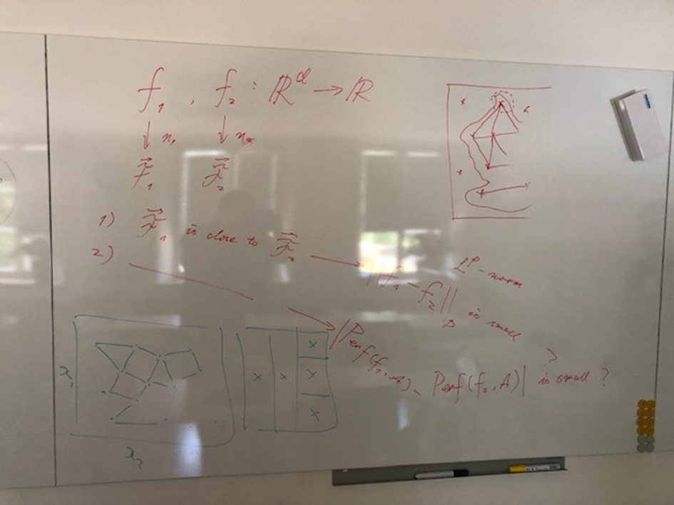
We were discussing the concept of “generalizability” in optimization theory, by which we intuitively mean the idea that if an optimization algorithm performs well on an optimization problem instance , it should also perform well on a sufficiently similar problem instance .
However, there are many open questions/loose ends in the above intuition. For instance, what we mean exactly by “similar problems (instances)” in the context of optimization.
-
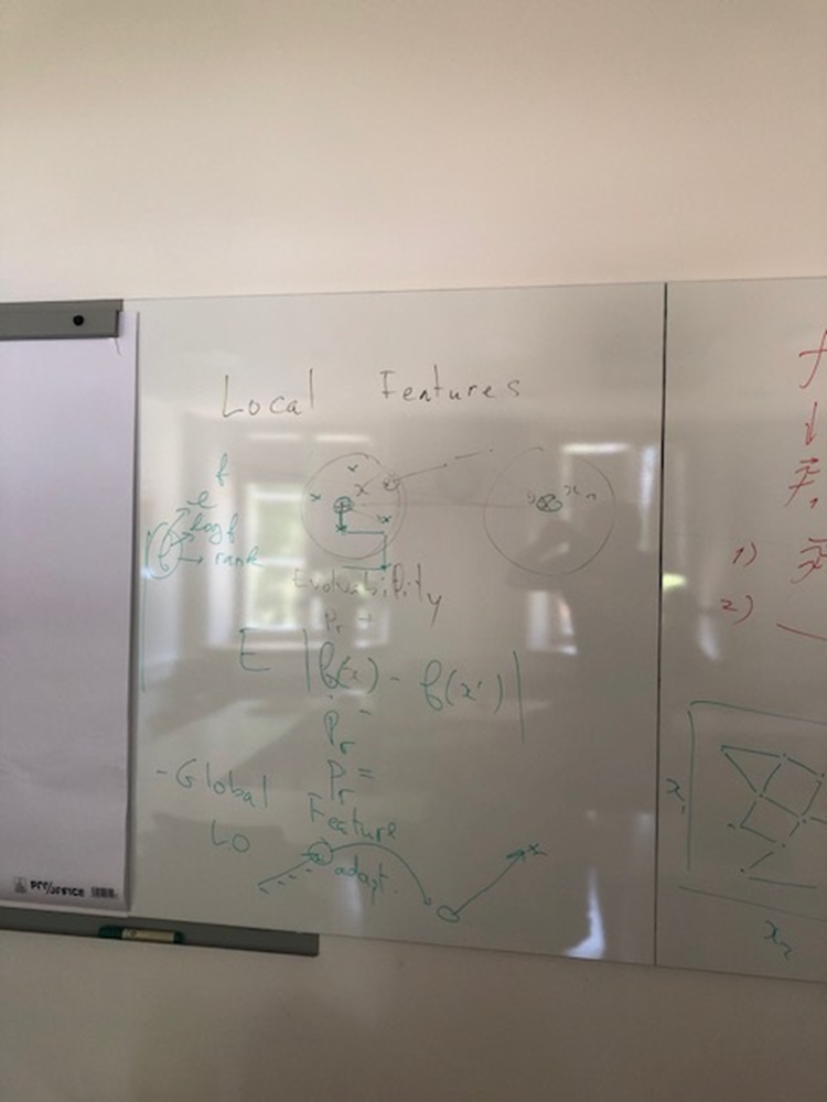
The concept of instance similarity could potentially be measured by distance in feature space, for which we would need features that describe instance characteristics appropriately.
-
We can distinguish between instance features (those that can be extracted from the instance data) and landscape features (which require sampling the fitness landscape involving neighborhood operators).
-
Interpretable features are important for experts/user to develop/understand the concept of generalizability, if possible.
-
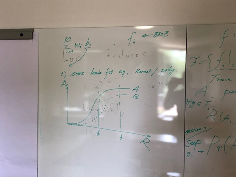
A large number of fitness landscape features have been already defined [2]: A single feature can not explain the whole search difficulty, several features can be linearly correlated, and on the contrary, a combination of features can be meaningful. Indeed, optimal relevant set of features is an open problem, and suppose to be problem domain dependent.
-
Feature normalization is important for developing such a distance measure.
-
It makes a big difference, whether we consider combinatorial or continuous/numerical optimization problems.
-
Information content, derived from random walk data on the decision space, was theoretically proven to be strongly related to the fluctuations of the gradient field of a continuous objective function [5].
-
We discussed the idea of whether neural networks could be used to automatically extract features. Some works are dedicated to this direction [6].
-
For continuous space with black-box optimization scenario, a sampling a search space is a way to discretize the continuous space. Based on this sampling, a neighborhood relation between sampled points can be defined in order to have discrete fitness landscape which approximate the original continuous one, and extract standard combinatorial fitness landscape features. Several sampling techniques can be used: static one such DoE [11], or adaptive one [9].
There are three main application domains for the features, namely (i) for algorithm selection/algorithm performance prediction, (ii) for defining instance similarity, and (iii) for defining instance hardness. The underlying assumption is that sufficiently similar problem instances would imply that an algorithm also yields similar performance on these instances. Based on that, we could come up, potentially, with a definition of “generalization”.
More (somewhat random) ideas that relate to these concepts:
-
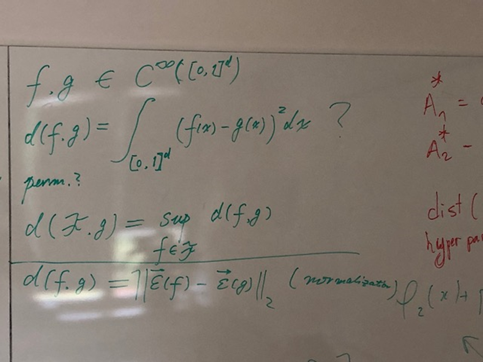
If we assume we have a set of training instances, we also have a set of baseline functions and could use a metric between sets of functions as a means to measure the similarity, e.g., Hausdorff distance. The most straightforward way to measure the similarity between two functions is the norm.
-
Notice that a measure of similarity based on features will depend on the scaling of the features values. So, it would be important to normalize the feature values (according to problem dimension, variance of values, maximum/minimum, quantity of information, etc.) to improve the meaningful of similarity measure.
-
We need to develop a cross-validation analogy with machine learning: enumerate or randomize all/many possible 80/20 splits.
-
Further open questions:
-
–
Which features should be used?
-
–
Which performance measures should be used?
-
–
Example in the combinatorial domain: QUBO.
-
–
Example in the continuous domain: BBOB (or a subset thereof).
-
–
-
(Probably approximately correct) PAC learning analogy:
-
–
Tuning hyperparameters of optimizers to problems.
-
–
Tuning hyperparameters of ML algorithms to data.
-
–
4.4.2 Feature-based generalizability
We assume the set of measurable functions (w.r.t. Borel sets on ) from to , where the domain for continuous black-box functions and for pseudo-Boolean functions (similar story for combinatorial problems). We shall assume the single-objective scenarios here (). Naturally, the -norm is defined for functions as follows:
We also consider a set of black-box optimization algorithms and an empirical performance measure , subject to maximization. Note that the empirical measure is essentially a random variable since it uses a finite set of independent runs/executions of an algorithm on a function to quantify the empirical performance.
For continuous black-box optimization problems/functions (which are infinite-dimensional objects), the -norm can only be computed with Monte Carlo method (convergence rate: according to CLT; is the number of function evaluations/data samples), which can be costly and unreliable. Hence, it is desirable to define some sample-efficient landscape features that are consistent with the -norm. Denoting by the numerical features of a function , we have the following intuitive criteria on assessing the appropriateness of numerical features:
-
1.
Consistency: : distances in function space is bounded by distances in feature space.
-
2.
Usefulness: : performance difference is bounded by feature difference;
-
3.
Effectiveness: for almost every function in , the convergence rate of (considered a statistical estimator) should not be slower than according to CLT, where is the number of function evaluations.
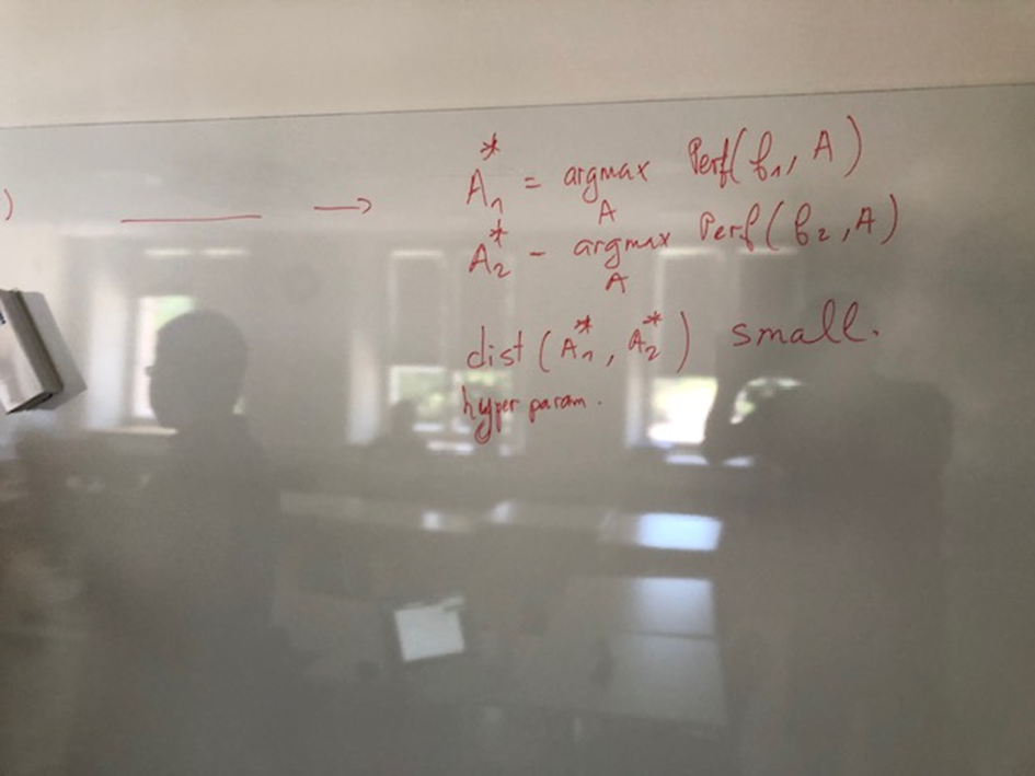
Going beyond this, one could be even more optimistic and assume that, if the two functions are similar, even the best performing algorithms (or at least hyperparameter settings for a given algorithm) for these two functions should be similar (e.g., in terms of their code, assuming they are programmed in the same programming language). This results in the following requirement (see also figure 2):
| (1) |
(although defining distance metric among algorithms is also a nontrivial task) Here, we assume that
| (2) |
A close enough goal, to start with, would be to say that the algorithm is not different, but for the same algorithm we are assuming the distance between their optimal hyperparameter configurations is small, i.e., and
| (3) |
4.4.3 Feature-free definition
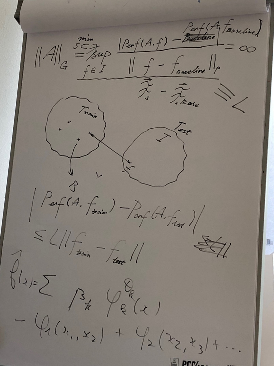
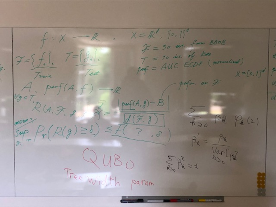
Another formulation attempt, as in figure 4, is based on the idea that we can use a training set of functions to “train” an algorithm and a test set to “test” whether generalizes thereto. In that case, we would require something like
| (4) |
where is the Hausdorff metric between the training and testing sets.
| (5) |
4.4.3.1 Example
To make things clearer, we were then trying to define an approach to test things in reality, both for the continuous domain and the binary domain . As test problem domains, we could use, say, training set to be 50 instances selected u.a.r. from BBOB, and test set to be 10 instances from BBOB, with AUC under the ECDF curve being the performance measure. Likewise, for the binary domain we had the idea to use QUBO problem formulations with a tree width parameter. A formulation following equation (4) would then, loosely formulated, look like
| (6) |
Now, imagine both and are sampled from training and testing function families, respectively. Then, we can compute the above ratio for multiple test sets, which are generated/sampled randomly from the testing family of functions. The empirical generalizability of algorithm from training family to can be calculated as , where are the ratio values obtained on multiple testing sets.
Since for a (infinite) function family, the above ratio can only be computed via a finite subset of functions, and therefore this ratio becomes a random variable. In this sense, it is natural/beneficial to provide a probabilistic formulation of generalizability (PAC-learning like):
| (7) |
for some upper bound function , to be developed in the future.
4.4.4 Papers of Interest and Related Work
-
Features for combinatorial multi-objective problems: [7]
-
An adaptive way to sample continuous single objective problems to create some possible features: [9]
-
MA-BBOB paper: [10]
-
Hyper-heuristics and cross-domain optimization [3, 4], are approaches that seek to increase the level of generality of optimization algorithms. They are practical algorithmic methods to solve complex combinatorial problems, and have not devoted much effort to quantifying the notion of generality of solvers.
References
- [1] Malan, K. & Engelbrecht, A. A survey of techniques for characterising fitness landscapes and some possible ways forward. Inf. Sci.. 241 pp. 148-163 (2013), https://doi.org/10.1016/j.ins.2013.04.015
- [2] Malan, K. A Survey of Advances in Landscape Analysis for Optimisation. Algorithms. 14, 40 (2021), https://doi.org/10.3390/a14020040
- [3] Burke, E., Gendreau, M., Hyde, M., Kendall, G., Ochoa, G., Özcan, E. & Qu, R. Hyper-heuristics: a survey of the state of the art. J. Oper. Res. Soc.. 64, 1695-1724 (2013), https://doi.org/10.1057/jors.2013.71
- [4] Ochoa, G., Hyde, M. & Others HyFlex: A Benchmark Framework for Cross-Domain Heuristic Search. Evolutionary Computation In Combinatorial Optimization (EvoCOP). 7245 pp. 136-147 (2012), https://doi.org/10.1007/978-3-642-29124-1%5C_12
- [5] Pérez-Salinas, A., Wang, H. & Bonet-Monroig, X. Analyzing variational quantum landscapes with information content. ArXiv Preprint ArXiv:2303.16893. (2023)
- [6] Stein, B., Long, F., Frenzel, M., Krause, P., Gitterle, M. & Bäck, T. DoE2Vec: Deep-learning Based Features for Exploratory Landscape Analysis. Companion Proceedings Of The Conference On Genetic And Evolutionary Computation, GECCO 2023, Companion Volume, Lisbon, Portugal, July 15-19, 2023. pp. 515-518 (2023), https://doi.org/10.1145/3583133.3590609
- [7] Liefooghe, A., Daolio, F., Vérel, S., Derbel, B., Aguirre, H. & Tanaka, K. Landscape-Aware Performance Prediction for Evolutionary Multiobjective Optimization. IEEE Trans. Evol. Comput.. 24, 1063-1077 (2020), https://doi.org/10.1109/TEVC.2019.2940828
- [8] Liefooghe, A., Vérel, S., Lacroix, B., Zavoianu, A. & McCall, J. Landscape features and automated algorithm selection for multi-objective interpolated continuous optimisation problems. GECCO ’21: Genetic And Evolutionary Computation Conference, Lille, France, July 10-14, 2021. pp. 421-429 (2021), https://doi.org/10.1145/3449639.3459353
- [9] Derbel, B., Liefooghe, A., Vérel, S., Aguirre, H. & Tanaka, K. New features for continuous exploratory landscape analysis based on the SOO tree. Proceedings Of The 15th ACM/SIGEVO Conference On Foundations Of Genetic Algorithms, FOGA 2019, Potsdam, Germany, August 27-29, 2019. pp. 72-86 (2019), https://doi.org/10.1145/3299904.3340308
- [10] Vermetten, D., Ye, F., Bäck, T. & Doerr, C. MA-BBOB: Many-Affine Combinations of BBOB Functions for Evaluating AutoML Approaches in Noiseless Numerical Black-Box Optimization Contexts. CoRR. abs/2306.10627 (2023), https://doi.org/10.48550/arXiv.2306.10627
- [11] Liefooghe, A., Verel, S., Lacroix, B., Zǎvoianu, A. & McCall, J. Landscape features and automated algorithm selection for multi-objective interpolated continuous optimisation problems. Proceedings Of The Genetic And Evolutionary Computation Conference. pp. 421-429 (2021)
5 Participants
-
David L. Applegate – Google – New York, US
-
Anne Auger – INRIA Saclay – Palaiseau, FR
-
Thomas Bäck – Leiden University, NL
-
Carolin Benjamins – Leibniz Universität Hannover, DE
-
Peter A. N. Bosman – CWI – Amsterdam, NL
-
Carola Doerr – Sorbonne University – Paris, FR
-
Katharina Eggensperger – Universität Tübingen, DE
-
Tobias Glasmachers – Ruhr-Universität Bochum, DE
-
Nikolaus Hansen – INRIA Saclay – Palaiseau, FR
-
Emma Hart – Edinburgh Napier University, GB
-
Holger H. Hoos – RWTH Aachen, DE
-
Pascal Kerschke – TU Dresden, DE
-
Lars Kotthoff – University of Wyoming – Laramie, US
-
Manuel López-Ibáñez – University of Manchester, GB
-
Mariapia Marchi – ESTECO SpA – Trieste, IT
-
Olaf Mersmann – TH Köln, DE
-
Boris Naujoks – TH Köln, DE
-
Gabriela Ochoa – University of Stirling, GB
-
Gorjan Popovski – Jozef Stefan Institute – Ljubljana, SI
-
Mike Preuß – Leiden University, NL
-
Lennart Schäpermeier – TU Dresden, DE
-
Ofer M. Shir – Tel-Hai College – Upper Galilee, IL
-
Kate Smith-Miles – The University of Melbourne, AU
-
Olivier Teytaud – Meta AI Research – Tournon-sur-Rhone, FR
-
Dirk Thierens – Utrecht University, NL
-
Tea Tusar – Jozef Stefan Institute – Ljubljana, SI
-
Konstantinos Varelas – Athens, GR
-
Sebastien Verel – Calais University, FR
-
Diederick Vermetten – Leiden University, NL
-
Vanessa Volz – modl.ai – Copenhagen, DK
-
Hao Wang – Leiden University, NL
-
Darrell Whitley – Colorado State University – Fort Collins, US
-
Stefan M. Wild – Lawrence Berkeley National Laboratory, US
![[Uncaptioned image]](x3.jpg)