Multiobjective Optimization on a Budget
Abstract
The Dagstuhl Seminar 23361 Multiobjective Optimization on a Budget carried on a series of seven previous Dagstuhl Seminars (04461, 06501, 09041, 12041, 15031, 18031, 20031) focused on Multiobjective Optimization. The original goal of this series has been to strengthen the links between the Evolutionary Multiobjective Optimization (EMO) and the Multiple Criteria Decision Making (MCDM) communities, two of the largest communities concerned with multiobjective optimization today. This seminar particularly focused on the case where the approaches from both communities may be challenged by limited resources.
This report documents the program and the outcomes of Dagstuhl Seminar 23361 “Multiobjective Optimization on a Budget”. Three major types of resource limitations were highlighted during the seminar: methodological, technical and human related. The effect of these limitations on optimization and decision-making quality, as well as methods to quantify and mitigate this influence, were considered in different working groups.
Keywords and phrases:
evolutionary algorithms, expensive optimization, few-shot learning, machine learning, optimization, simulationSeminar:
September 3–8, 2023 – http://www.dagstuhl.de/233612012 ACM Subject Classification:
Computing methodologies Machine learning ; Computing methodologies Neural networks ; Mathematics of computing Evolutionary algorithms ; Theory of computation Mathematical optimization ; Computing methodologies Computational control theoryCopyright and License:
![[Uncaptioned image]](x1.png) Except where otherwise noted, content of this report is licensed under a
Creative Commons BY 4.0 International license
Except where otherwise noted, content of this report is licensed under a
Creative Commons BY 4.0 International license
1 Executive Summary
Richard Allmendinger (University of Manchester, GB)
Carlos M. Fonseca (University of Coimbra, PT)
Serpil Sayin (Koc University – Istanbul, TR)
Margaret M. Wiecek (Clemson University, US)
License: ![[Uncaptioned image]](x2.png) Creative Commons BY 4.0 International license © Richard Allmendinger, Carlos M. Fonseca, Serpil Sayin, and Margaret M. Wiecek
Creative Commons BY 4.0 International license © Richard Allmendinger, Carlos M. Fonseca, Serpil Sayin, and Margaret M. Wiecek
Multiobjective optimization (MO), a discipline within systems science that provides models, theories, and methodologies to address decision-making problems under conflicting objectives, has a myriad of applications in all areas of human activity ranging from business and management to engineering. This seminar is a result of the desire to continue to make MO useful to society as it faces complex decision-making problems and experiences limited resources for decision making. Of particular interest are processes that evolve competitively in environments with scarce resources and lead to decision problems that are characterized by multiple, incommensurate, and conflicting objectives, and engage multiple decision-makers. Viewing optimization and decision making as the complementary aspects of the multiobjective paradigm, the seminar set out to focus around three major types of resource limitations: methodological (e.g., number of solution evaluations), technical (e.g., computation time, energy consumption), and human related (e.g., decision maker availability and responsiveness). The effect of these limitations on optimization and decision-making quality, as well as methods to quantify and mitigate this influence, were of particular interest. Ideas related to modelling, theory, algorithm design, benchmarking, performance metrics, and novel applications of MO under budget constraints were discussed.
To initiate a discussion among the participants on how to address challenges of MO under a budget, the organizers presented specific research directions at the beginning of the seminar. These directions along with their highlights are described below.
-
Model reduction: In the MO problem not all functions may be of interest to the decision maker (DM) or not all objectives may be in conflict with each other. Under a limited budget, it is of interest to make the original problem simpler by removing unnecessary objective functions while the solution set remains unchanged. Another reason to reduce the problem is its size. MO problems with four or more criteria bring computational and decision-making challenges that are not typical when the number of objectives is lower.
-
Model decomposition and coordination-based decision making: If a reduction of the objectives is not possible, then the solution of the overall MO problem in its entirety may be challenging or even impossible to obtain. In this situation, decomposition of the MO problem into a set of MO subproblems with a smaller number of criteria becomes appealing provided solving the subproblems can be coordinated and related to solving the original problem. When the MO problem is decomposed while computation of the overall solution set is possible, the decomposition goal is to enhance capability of making coordinated tradeoff decisions by working in lower dimensional spaces, which decreases the cognitive burden on DMs. Otherwise, if computation of the overall solution set is not possible, the decomposition goal becomes more challenging since the intention is to coordinate the subproblems’ solution sets to construct the overall set and to facilitate decision making in a similar way.
-
Representation of the optimization solution set: It is of interest to design cost-effective methods for obtaining a complete or partial description of the Pareto set. An exact description of this set might be available analytically as a closed-form formula, numerically as a set of points, or in mixed form as a parametrized set of points. Unfortunately, for the majority of MO problems, it is not easy to obtain an exact description of the solution set that includes typically a very large number or infinite number of points. Even if it is theoretically possible to find these points exactly, this is often computationally challenging and expensive, and therefore is usually abandoned. On the other hand, if it is possible to obtain the complete solution set, one might not be interested in this task due to overflow of information. Another reason for approximating the solution set, rather than finding the solution set exactly, is that many real-world problems (e.g., in engineering) cannot be completely and correctly formulated before a solution procedure starts. Since the exact solution set is very often not attainable, an approximated description of the solution set becomes an appealing alternative.
-
Surrogate-assisted optimization: The combination of evolutionary MO (EMO) algorithms with efficient computational models, often known as metamodels or surrogates, has become a common approach to approximate outcomes of a time-consuming, expensive, and/or resource intense simulation or physical experiment, and thus to tackle problems with a limited budget. Surrogate-assisted (SA) methods vary in aspects such as the use of the metamodel (e.g., different models for different objective functions or one model for all objective functions), type of metamodel (e.g., Gaussian process, radial basis neural network, etc.), how the metamodel is updated (e.g., expected improvement, expected hypervolume improvement), and training time of the metamodel. In particular, the combination of optimization with Gaussian process approximation, known as Bayesian optimization, is a recent trend to efficiently deploy data in model development.
-
Multistage optimization: In real-world applications, problem data does not always become available all at once, but at different points in time until a final decision needs to be made. In particular, waiting until all the required data is available may not leave enough time to run the optimization process on the whole problem and successfully compute a final decision. In addition, it is often possible to model the uncertainty associated with the yet unknown data given the data that is already known, at least to some extent. Two-stage (and, more generally, multi-stage) approaches to optimization reformulate the original problem as a number of sub-problems to be solved sequentially, in such a way that the last problem(s) in the sequence can effectively be solved in the (short) time available.
-
Preference acquisition and communication with the decision maker: The ultimate goal in MO is to serve one or multiple DMs whose goal is to come up with a single most preferred solution from among the ones that are available. Given an optimization model, DM’s preferences may be incorporated prior to, during or after employing a solution procedure. In particular, interactive methods require the DM’s involvement in the solution process during which they reveal their preferences based on the presented information. Under a limited budget, communication with the DM shall be designed effectively and economically.
-
Benchmarking of algorithms: SA methods are considered as the method of choice to tackle problems subject to a limited budget in terms of function evaluations. However, SA methods are not often compared to widely different alternatives (e.g., different kernels and distance measures, non-SA methods, etc.), and are often tested on narrow sets of problems (multimodal, low-dimensional, static, deterministic, unconstrained, and continuous functions) and rarely on real-world problems, which makes it difficult to assess where (or if) these methods actually achieve state-of-the-art performance in practice. Moreover, several aspects in the design of SA algorithms vary across implementations without a clear recommendation emerging from current practices, and many of these design choices are not backed up by authoritative test campaigns. This seminar topic aimed to raise awareness and hence a push to more work being carried out on developing benchmarking guidelines for SA algorithms.
In response to the presented research directions, some participants found research topics of interest among those suggested by the organizers. These topics included model reduction, decomposition and coordination, solution set representation, and surrogate modeling. Other participants proposed different topics that also targeted the theme of MO under a budget. Those topics included design of experiments for MO, correlations in MO, and design of evolutionary algorithms. Overall, seven research topics were proposed and pursued.
Independently of developing and forming research topics, a collection of eight talks were given during the seminar. Two of the speakers were considered “invited” because they were asked before the seminar to give a talk. These talks addressed two of the research directions initiated by the organizers. The other speakers, being inspired by the ongoing seminar, proposed talks that were integrated daily into the seminar program. The invited and contributed talks kept the seminar in balance ensuring ample time for working in groups.
During the seminar the schedule was updated on a daily basis to maintain flexibility in balancing time slots for the invited and contributed talks, discussions, and working group sessions. The working groups were established on the first day in an interactive fashion. Starting with three large working groups focused around the three central topics of the seminar (methodological, technical, and human-related resource limitations), participants were invited to formulate their favorite topics and most important challenges. The three initial groups split to eventually form eight groups by the end of the seminar. During the week the participants were allowed to change the working groups based on their research interest. The abstracts of the delivered talks and the extended abstracts of the working groups can be found in the subsequent chapters of this report.
Further notable events during the week included: (i) a hike that took place on Wednesday afternoon, (ii) a session allowing the participants to share the details of upcoming professional events in the research community, (iii) a joint session with the participants of the concurrent seminar 23362 “Decision-Making Techniques for Smart Semiconductor Manufacturing” and (iv) an informal get together on Thursday evening.
Offers and Needs Market
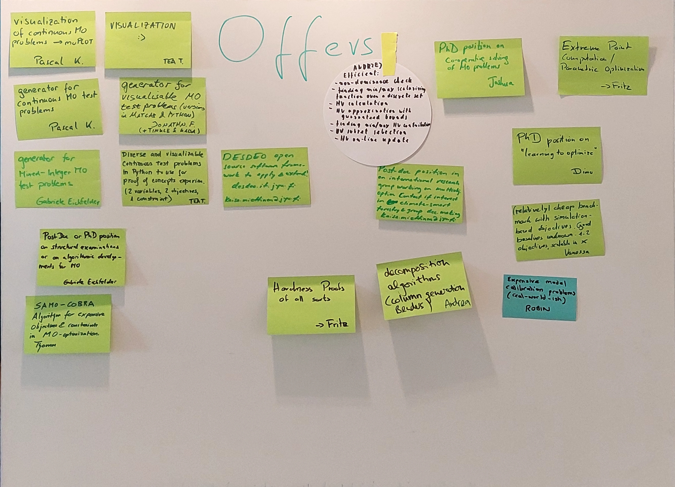
An Offers Needs Market ran throughout the entire week. The participants could write their research offers and needs regarding MO on note paper in different colors and post them on pin boards (see Fig. 1) to attract or find a possible collaborator. Participants discussed potential collaboration opportunities during the coffee breaks and after hours.

Outcomes
The outcomes of each of the working groups can be seen in the sequel.
The organizers have arranged a special issue of the Journal of Multi-Criteria Decision Analysis entitled “Multiobjective Optimization on a Budget” for which they will serve as Guest Editors. This issue will be an outlet for papers authored and submitted by the seminar’s participants as well as by researchers world-wide.
This seminar resulted in a very insightful, productive and enjoyable week. It has already led to first new results, cooperations and research topics.
Acknowledgements
The organizers would like to express their appreciation to the Dagstuhl Office and its helpful and patient staff for their professional support and smooth cooperation; huge thanks to the organizers of the previous seminars in this series for setting us up for success; and thanks to all the participants, who worked hard and were amiable company all week.
In a later section, we also give special thanks to Margaret Wiecek as she steps down from the organizer role.
2 Table of Contents
3 Overview of Talks
3.1 Objective Space Methods: Pareto Front Approximations on a Budget
Kathrin Klamroth (Universität Wuppertal, DE), Kerstin Dächert (HTW Dresden, DE), Daniel Vanderpooten (University Paris-Dauphine, FR)
License: Creative Commons BY 4.0 International license © Kathrin Klamroth, Kerstin Dächert, and Daniel Vanderpooten
Joint work of: Kerstin Dächert, Kathrin Klamroth, Renaud Lacour, Daniel Vanderpooten
Objective space methods usually rely on (often recursive) decompositions of the objective space, and on the associated formulation of problem scalarizations that are solved by available (single-objective) solvers. The number of solver calls and the complexity of the scalarizations are decisive for the computational effort and may be subject to time, energy or cost constraints. We will briefly review objective space methods and initiate a discussion on the impact of pre-specified budget constraints on the algorithmic choices.
References
- [1] K. Dächert. C++ Implementation of the Defining Point Algorithm on github (Version 2023). https://github.com/kerstindaechert/DefiningPointAlgorithm
- [2] K. Dächert and K. Klamroth. A linear bound on the number of scalarizations needed to solve discrete tricriteria optimization problems. Journal of Global Optimization 61(4):643-676, 2015
- [3] K. Dächert, K. Klamroth, R. Lacour and D. Vanderpooten. Efficient computation of the search region in multi-objective optimization. European Journal of Operational Research 260(3):841-855, 2017
- [4] K. Klamroth, R. Lacour and D. Vanderpooten. On the representation of the search region in multi-objective optimization. European Journal of Operational Research 245(3):767-778, 2015
- [5] R. Lacour, K. Klamroth and C.M. Fonseca. A box decomposition algorithm to compute the hypervolume indicator. Computers & Operations Research 79:347-360, 2017
- [6] S. Tamby and D. Vanderpooten. Enumeration of the nondominated set of multiobjective discrete optimization problems. INFORMS Journal on Computing 33(1):72-85, 2000
3.2 Perspectives to Dealing with Computationally Expensive Multiobjective Optimization Problems
Kaisa Miettinen (University of Jyväskylä, FI)
License: Creative Commons BY 4.0 International license © Kaisa Miettinen
Multiobjective optimization methods are needed since real-life problems typically have several conflicting objective functions to be optimized simultaneously. To find the most preferred Pareto optimal solution as the final one to be implemented in practice, we typically need preference information from a domain expert, a decision maker (DM).
We concentrate on interactive methods, where the DM takes actively part and directs the solution process with one’s preference information. One can learn and gain insight about the problem and also adjust preferences while learning. Importantly, one can concentrate on solutions that seem most promising and avoid high cognitive load of analyzing too much information at a time.
In real applications, function evaluations may be expensive and we outline different approaches. The first is to generate a representative set of Pareto optimal solutions in advance and create a surrogate problem that is computationally inexpensive. In the second approach, we replace a scalarizing function that a multiobjective optimization method employs by a computationally inexpensive metamodel. The third approach is to fit a metamodel to each computationally expensive objective function. Appropriate approaches are also needed if constraint functions are expensive or functions in the problem to be solved have different latencies.
By speeding up calculations, we avoid keeping the DM waiting when applying interactive methods. But the presence of the human DM means that attention must be paid to the understandability and amount of information expected from the DM. We briefly outline pros and cons of some methods and mention further challenges.
3.3 Surrogate model guided optimization of expensive black-box multiobjective problems
Juliane Mueller (NREL – Golden, US)
License: Creative Commons BY 4.0 International license © Juliane Mueller
Many engineering applications require the simultaneous optimization of multiple conflicting objective functions. Often, these objective functions are evaluated using highly accurate computer simulations that are computationally too expensive to be evaluated hundreds or thousands of times during optimization. Thus, the goal is to find good approximations of the Pareto front using as few of these expensive simulations as possible. Here, we describe an optimization approach based on surrogate models and diverse sampling strategies to accelerate the search for the Pareto solutions. We use a separate surrogate model for approximating each objective function and then we use the surrogate models to inform where additional expensive simulations should be run. The surrogate models are updated in an active learning framework whenever new information from the expensive simulations becomes available. The sampling strategies aim at balancing local improvements of the approximate Pareto front and global exploration to identify the extrema and fill in large gaps of the approximate Pareto front. We demonstrate on a large set of benchmark problems the effectiveness of the method for finding good approximations of the Pareto front.
3.4 Fast Pareto Optimization Using Sliding Window Selection
Frank Neumann (University of Adelaide, AU)
License: Creative Commons BY 4.0 International license © Frank Neumann
Joint work of: Frank Neumann, Carsten Witt
Pareto optimization using evolutionary multi-objective algorithms such as the classical GSEMO algorithm has been widely applied to solve constrained submodular optimization problems. A crucial factor determining the runtime of the used evolutionary algorithms to obtain good approximations is the population size of the algorithms which grows with the number of trade-offs that the algorithms encounter. In this paper, we introduce a sliding window speed up technique for recently introduced algorithms. We prove that our technique eliminates the population size as a crucial factor negatively impacting the runtime of the classical GSEMO algorithm and achieves the same theoretical performance guarantees as previous approaches within less computation time. Our experimental investigations for the classical maximum coverage problem confirms that our sliding window technique clearly leads to better results for a wide range of instances and constraint settings.
3.5 Towards decision analytic workflows for real-world problems: Simulation model calibration and multi-objective optimization on a shared evaluation budget
Robin Purshouse (University of Sheffield, GB)
License: Creative Commons BY 4.0 International license © Robin Purshouse
Joint work of: Oliver P. H. Jones, Jeremy E. Oakley, Robin C. Purshouse
Real-world multi-objective optimization problems sometimes include evaluation functions that rely on computationally expensive simulation models. These types of problems typically constrain the optimization budget to a relatively small number of candidate solutions, e.g. 500-5000. An often-overlooked issue in such problems is that the simulations (i.e. evaluation functions) typically require the calibration of their parameters before they are ready for use in solving a particular problem instance. The simulations can also contain discrepancies – e.g. simplifications in the representation of the physics of the problem–that affect the robustness of solution evaluations. Simulation model calibration is a research field in its own right and concerns itself with inference of model parameters and model discrepancy structures. Inference is typically computational in nature, uses Bayesian methods, and involves the evaluation of sampled candidate parameterisations and discrepancy terms via the simulation model – i.e. it also involves evaluation functions and a constrained evaluation budget. To improve the efficiency of the inference process, low fidelity “emulators”, often Gaussian processes, are estimated using data sampled from the high fidelity model, closely mirroring the use of surrogate models in optimization workflows. Perhaps surprisingly, very little research has been conducted into the joint problem of simulation model calibration and multi-objective optimization based on such models. How should an evaluation budget best be allocated to the two activities, how should they be sequenced, and how can synergies between the two be exploited? This presentation introduces this novel topic, demonstrates some illustrative benchmark problems, and sketches some tentative solution architectures.
Acknowledgements: Robin Purshouse is supported by SIPHER (MR/S037578/1), a UK Prevention Research Partnership funded by the UK Research and Innovation Councils, the Department of Health and Social Care (England) and the UK devolved administrations, and leading health research charities https://ukprp.org/. Oliver Jones was supported by the UK Engineering and Physical Sciences Research Council.
References
- [1] Jones OPH, Oakley JE, Purshouse RC, Toward a unified framework for model calibration and optimisation in virtual engineering workflows, 2019 IEEE International Conference on Systems, Man and Cybernetics (SMC), 2019, pp. 3148–3153.
- [2] Jones O, A framework for combining model calibration with model-based optimization in virtual engineering design workflows, PhD thesis, University of Sheffield, 2021.
- [3] Jones OPH, Oakley JE, Purshouse RC, Simulation-based engineering design: solving parameter inference and multi-objective optimization problems on a shared simulation budget, 2021 IEEE International Conference on Systems, Man, and Cybernetics (SMC), 2021, pp. 1399–1405.
3.6 Efficient Approximation of Expected Hypervolume Improvement Using Gauss-Hermite Quadrature
Alma Rahat (Swansea University, GB)
License: Creative Commons BY 4.0 International license © Alma Rahat
Joint work of: Alma A. M. Rahat, Tinkle Chugh, Jonathan E. Fieldsend, Richard Allmendinger, Kaisa Miettinen
Many methods for performing multi-objective optimisation of computationally expensive problems have been proposed recently. Typically, a probabilistic surrogate for each objective is constructed from an initial dataset. The surrogates can then be used to produce predictive densities in the objective space for any solution. Using the predictive densities, we can compute the expected hypervolume improvement (EHVI) due to a solution. Maximising the EHVI, we can locate the most promising solution that may be expensively evaluated next. There are closed-form expressions for computing the EHVI, integrating over the multivariate predictive densities. However, they require partitioning of the objective space, which can be prohibitively expensive for more than three objectives. Furthermore, there are no closed-form expressions for a problem where the predictive densities are dependent, capturing the correlations between objectives. Monte Carlo approximation is used instead in such cases, which is not cheap. Hence, the need to develop new accurate but cheaper approximation methods remains. Here we investigate an alternative approach toward approximating the EHVI using Gauss-Hermite quadrature. We show that it can be an accurate alternative to Monte Carlo for both independent and correlated predictive densities with statistically significant rank correlations for a range of popular test problems.
3.7 Problem decomposition in biobjective optimisation
Andrea Raith (University of Auckland, NZ)
License: Creative Commons BY 4.0 International license © Andrea Raith
Joint work of: Matthias Ehrgott, Ruchard Lusby, Andrew Mason, Siamak Moradi, Melanie Reuter-Oppermann, Ali Sohrabi Yousefkhan
Decomposition techniques for optimisation problems have significantly improved the ability to solve problems of ever-increasing complexity and problem size by decomposing a complex optimisation problem into related smaller ones. The premise of a decomposition technique is to omit parts of the problem that are unlikely to influence the final solution, and iteratively include, as needed, the parts which will have an impact. Many real-world problems must be formulated with two or more objectives and solving such multiobjective optimisation problems means identifying sets of so-called efficient solutions representing available trade-offs. Different solution algorithms for biobjective linear programmes (BLPs) will be discussed in this talk. Building on a biobjective (parametric) version of the well-known simplex algorithm, different decomposition approaches are presented here. One approach, also known as column generation, is to omit some or all variables (corresponding to columns of the constraint matrix) from the original optimisation problem and then iteratively re-introduce them into the problem. An alternative approach, known as Benders decomposition, separates decision variables into different stages and related optimisation problems, and then dynamically adds constraints into the first-stage formulation to capture the full problem. We present theoretical developments and algorithms that adapt these ideas into decomposition techniques for BLPs. We will also briefly discuss initial developments of a so-called math-heuristic approach that combines exact optimisation concepts with a neighbourhood search heuristic that can be used instead of an exact column generation approach.
3.8 A Visualization-Aided Approach to Solving Tri-Criterion Portfolio Problems
Ralph E. Steuer (University of Georgia – Athens, US)
License: Creative Commons BY 4.0 International license © Ralph E. Steuer
Joint work of: Ralph E. Steuer, Sebastian Utz
This talk contains no text or equations, only graphs. It is about (1) how much more enormously difficult it is to identify one’s best point on an efficient surface than on an efficient frontier and (2) how, on problems in which one objective appears to carry more influence, a visually assisted approach utilizing a new type of line stretched across the efficient set can be applied. Of course, the approach works best the less severely disordered the efficient surface is. A non-trivial tri-criterion portfolio optimization problem is used to illustrate throughout.
3.9 Multi-objective Branch-and-Bound on a Budget
Michael Stiglmayr (Universität Wuppertal, DE)
License: Creative Commons BY 4.0 International license © Michael Stiglmayr
Joint work of: Julius Bauß, Michael Stiglmayr
In this talk we discuss modifications of multi-objective branch-and-bound to diversify solutions and yield a good approximation of the non-dominated set when only limited computation time is available. It is crucial not only to find efficient solutions in early stages of the algorithm but also to find a set of solutions whose images are close to and well distributed along the non-dominated frontier. In particular the adaptation of branching and queuing of sub-problems seems to be important. We use, e.g., the hypervolume indicator as a measure for the gap between lower and upper bound set to implement a multi-objective best-first strategy. Moreover, gap measure indicate the solution quality when prematurely stopping the branch-and-bound algorithm.
References
- [1] Bauß, J., Stiglmayr, M.: Augmenting bi-objective branch and bound by scalarization-based information (2023), https://arxiv.org/abs/2301.11974
- [2] Bauß, J., Stiglmayr, M.: Adapting branching and queuing for multi-objective branch and bound (2023), https://arxiv.org/abs/2311.05980
4 Working groups
4.1 Decoupled Design of Experiments for Multi-objective Optimisation on a Budget
Mickaël Binois (INRIA – Sophia Antipolis, FR), Jürgen Branke (University of Warwick, GB), Jonathan Fieldsend (University of Exeter, GB), Robin Purshouse (University of Sheffield, GB)
License: Creative Commons BY 4.0 International license © Mickaël Binois, Jürgen Branke, Jonathan Fieldsend, and Robin Purshouse
4.1.1 Introduction
Fundamental to the performance of surrogate-based optimisation frameworks is the need to construct an initial model based on a carefully selected set of initial designs, and any prior system knowledge. This is both in the case of Bayesian optimisation, which used and iteratively update model(s) mapping decision vectors to predicted performance criteria values, and for evolutionary computation approaches which involving surrogates. The selection and construction of initial designs, which are often treated separately to the decision vectors queried during the subsequent optimisation process, are usually referred to as the design of experiments (or DoE for short). This is because these decision vectors are selected to – in some fashion – be maximally informative on the global underlying process, rather than being biased towards particular regions.
Without any prior information regarding the properties of the objective function(s) such DoE for model fitting are commonly based around space filling sequences such as Latin hypercube sampling [9] or Sobol sequences [10], as purely random sampling tends to naturally result in clusters, which do not serve model fitting well, particularly when the budget for sampling is tight.
Where there are multiple criteria being modelled, this leads to an interesting and under-explored question: should one evaluate all initial designs fully, or selectively evaluate a subset of objectives per design, allowing a greater number of locations to be partially evaluated when building the model(s)? A few works have looked at decoupling objective evaluations during the search process – particularly where there are different costs associated with each objective, but this can also be advantageous where there is a difference in the complexity of the functions being modelled (e.g. one being smooth slowly changing, the other being rugged and fast changing). As such, this appears to be a promising direction for further investigation and research, as even small improvements in such areas can effectively lead to large savings for expensive optimisation problems.
4.1.2 Related Work
A small number of existing works have considered decoupled and/or cost-aware multi-objective optimisation – some of which have considered these factors during the initial DoE phase. Below we discuss the most relevant approaches. A wider survey on the topic of objectives with different costs can be found in [1].
Hernández-Lobato and colleagues proposed the Predictive Entropy Search for Multi-Objective Bayesian Optimization (PESMO) method [6]. PESMO uses predictive entropy search as the acquisition function. This function represents each objective using an additive component, which enables a decoupled evaluation approach to be adopted. The approach was subsequently extended to also consider constraints (again where decoupling is possible) [5].
Suzuki et al. developed the Pareto-frontier entropy search (PFES) approach [11]. PFES is also an entropy approach but considers the entropy in objective-space rather than decision-space, which is computationally simpler. This method also includes cost in evaluating the objectives by including cost in the denominator of the acquisition function. Like PESMO, the approach is easily extended to consider decoupled evaluations.
Iqbal and colleagues proposed the Flexible Multi-Objective Bayesian Optimization (FlexiBo) algorithm [7]. The approach uses a decoupled evaluation in the Bayesian optimisation run but uses a coupled initial DoE procedure. FlexiBo includes two main features: (1) a new acquisition function that is the expected change in hypervolume if only one objective function is evaluated, divided by the cost of this function evaluation; and (2) a confidence region in the objective space for the partially evaluated points. The estimated cost of evaluating each objective is updated each time the objective is evaluated – this is a mean estimate of the cost (treating any observed variability as occurring at random).
Most recently, Buckingham et al. extended the multi-attribute Knowledge Gradient [2] to the case where objectives can be evaluated independently [3]. The authors demonstrate the benefit of independent evaluation not only when the computational times for objectives differ, but also when the lengthscales of the modelled landscapes (which determine the smoothness of the landscape) differ.
A slightly different problem is considered in [8], where one objective is much cheaper (essentially free) to evaluate than the other. They directly incorporate evaluation of the cheap objectives into a pair of hypervolume-based acquisition functions for BO. Consequently, the cheap objectives are evaluated many times while the acquisition function is optimized.
A summary of the different approaches is shown in Table 1, highlighting which methods feature decoupled and cost-aware acquisition functions during the initial DoE, the subsequent optimisation run, or both phases.
| Design of experiments | Optimisation | ||||
| Approach | Decoupled? | Cost-aware? | Decoupled? | Cost-aware? | Acquisition function |
| PESMO [6] | ✓ | ✗ | ✓ | ✗ | predictive entropy search |
| PFES [11] | ✗ | ✗ | ✓ | ✓ | cost-weighted Pareto frontier entropy |
| FlexiBO [7] | ✗ | ✗ | ✓ | ✓ | cost-weighted objective space entropy |
| C-MOKG [3] | ✗ | ✗ | ✓ | ✓ | cost-weighted multi-objective knowledge gradient |
4.1.3 New analyses by the working group
4.1.3.1 Initial DoE when evaluations are decoupled
The costs of the objectives are assumed to be the same for now.
Goal: studying the effect on coupled vs. decoupled designs of experiments (DoE) on the uncertainty on the Pareto front.
To this end, we experiment on Gaussian process models (GPs). More precisely, we generate samples from a Gaussian process model and use it as the ground truth. The hyperparameters are supposed to be known to remove the effect of inference. Hence there is no model mismatch. Examples of outcome are given in Figure 2.
Next, to measure the uncertainty on the Pareto front associated with the fitted GPs, we rely on the so called Vorob’ev deviation (VD), a set based variance measure, see Algorithm 1 for a pseudo code and, e.g., [4] for the details. The reference point used for hypervolume computations is taken to be . An example is provided in Figure 3, where the DoE for the first objective is the same while the second one is either coupled or decoupled. One visible effect is that when both objectives are jointly evaluated, the area that is dominated (attainment value = 1) is larger. This is probably because in the decoupled case, solutions are never surely dominated (even though the domination probability is extremely low).
We compare VD values of different setups for the coupled and decoupled case:
-
the DoE for the first objective is either uniformly sampled or is a maximin Latin hypercube design;
-
the DoE for the second objective is the same as the first objective (coupled case), uniformly sampled or an LHS augmenting the DoE of the first objective.
Figure 4 shows the results. Comparing the top row (both initial designs uniformly sampled) with the middle row (an augmenting LHS used to complement the first uniform DoE), there seems to be not much difference. However, the bottom row (first design is sampled with LHS, second uses augmenting LHS) shows a significant improvement of the Vorob’ev deviation of either the coupled (red dots) or decoupled (box plots) sampling. Clearly, a space-filling design improves our estimate of the Pareto front, but it seems not sufficient to only make the design of the second objective space-filling.
Note that with respect to the Vorob’ev deviation, when at least one of the designs is random (first two rows, first two columns), the red dots are sometimes above and sometimes below the median of the boxplots, while the red dots are mostly below the median of the boxplots in the bottom row (full space-filling design). This indicates that at least if a space-filling design is used, decoupled sampling is worse than coupled sampling, possibly due to the effect mentioned above on the size of the known dominated region. Note, however, that in these experiments we assume equal cost of sampling the two objectives, and equal lengthscales of the two objectives. As we see later, in other cases decoupling may be beneficial.
The results look slightly different when considering the expected product of the standard deviations of the GP (right column), which is an indication of the accuracy of the estimation quality of the models over the entire search space, rather than the Pareto frontier. Here, the first two rows show a clear benefit of decoupled sampling. However, this benefit seems to disappear once both objectives are sampled using space-filling designs (third row).
4.1.3.2 Initial DoE when evaluations have different costs
Now let us assume the cost is different between different objectives and (etc). The first tasks are to define the total time budget for experiments and get relative costs of , , , . We will then consider a number of alternative approaches to DoE, including a coupled baseline.
-
1.
(Coupled) Both functions evaluated at once.
-
2.
(Decoupled naive) Both functions evaluated the same number of times, but at differing locations. (generated by Augmented LHS)
-
3.
(Decoupled) The allocation of total budget to the two functions depends on lengthscales and relative costs, according to Eq. 1. Objectives with smaller lengthscales and smaller cost are sampled more often.
Considering how to split the computational budget, let us consider the simplest case of optimising a (weighted) sum of two objectives. In such a case, if we want to minimise integrated mean squared prediction error (IMSPE), then it is not possible to improve beyond coupled sampling, as the variances of the two functions just add up, and the optimal design for each function would be the same. However, if the costs or lengthscales are different, then we could use IMSPE to determine an appropriate allocation of the budget to the two functions as follows:
| (1) |
where is the total budget, is the number of samples allocated to objective , and are the cost of evaluating objective .
As in the previous section, we rely on GP samples to define a ground truth. We also assume some known values of the lengthscales of the objectives: for the first, for the second. We start with four initial designs for each objective in the various cases, then 26 decoupled evaluations are performed. We only compare the ‘coupled’, ‘naive’ and ‘decoupled’ strategies. The results are in Figure 5. First, from the IMSPE results, we observe that the values for objective 1 and 2 are different (importantly, the GP variances are equal here), due to the different lengthscales. The naive baseline always performs worst. Then, in the same cost case, there is no change between the coupled and decoupled case. As the cost of increases, the effect is that the IMSPE of is reduced faster compared to , with no strong detrimental effect on for the same total cost. The outcome is that it is reasonable to sample more , in a ratio that only depends on the lengthscales and relative cost.
4.1.4 Discussion and future research ideas
In this report, we have examined the possibility of improving the quality of the surrogate models obtained through a DoE in case of multi-objective optimisation where the evaluation of the different objectives can be decoupled. We found that for the case of equal lengthscales, decoupling the evaluations (i.e., evaluating different solutions on different objectives) did tend to worsen the quality of the Pareto front estimate as measured by Vorob’ev deviation. However, when objectives had different costs and/or lengthscales, decoupling could improve results substantially in terms of total IMPSE.
In the future, we plan to investigate also other sampling strategies such as taking into account the posterior of the first objective when deciding where to evaluate the second objective, or to learn each objective function’s lengthscale and cost on the fly.
4.1.5 Acknowledgements
This report benefited from wider discussions within the “Surrogates” working group of the Dagstuhl Seminar 23361 Multiobjective Optimization on a Budget. This group’s members included Thomas Bäck, Mickaël Binois, Jürgen Branke, Jonathan Fieldsend, Ekhine Irurozki, Pascal Kerschke, Boris Naujoks, Robin Purshouse, Tea Tusar, Vanessa Volz, Hao Wang and Kaifeng Yang.
References
- [1] Richard Allmendinger and Joshua Knowles, Heterogeneous Objectives: State-of-the-Art and Future Research, arXiv preprint arXiv:2103.15546, 2, 2021
- [2] Raul Astudillo and Peter Frazier, Multi-attribute Bayesian optimization under utility uncertainty In: Proceedings of the NIPS Workshop on Bayesian Optimization, 172, 2017.
- [3] Jack M. Buckingham, Sebastian Rojas Gonzalez and Juergen Branke, Bayesian Optimization of Multiple Objectives with Different Latencies, arXiv preprint arXiv:2302.01310, 2023.
- [4] Mickaël Binois, David Ginsbourger and Olivier Roustant, Quantifying uncertainty on Pareto fronts with Gaussian process conditional simulations, European Journal of Operational Research, 243(2), 386–394, 2015.
- [5] Eduardo C Garrido-Merchán and Daniel Hernández-Lobato, Predictive Entropy Search for Multi-objective Bayesian Optimization with Constraints, Neurocomputing, 361, 50–68, 2019.
- [6] Daniel Hernández-Lobato, Jose Hernandez-Lobato, Amar Shah and Ryan Adams, Predictive entropy search for multi-objective Bayesian optimization, In: International Conference on Machine Learning, 1492–1501, PMLR, 2016.
- [7] Md Shahriar Iqbal, Jianhai Su, Lars Kotthoff and Pooyan Jamshidi, FlexiBO: A Decoupled Cost-Aware Multi-Objective Optimization Approach for Deep Neural Networks, Journal of Artificial Intelligence Research, 77, 645–682, 2023.
- [8] Nasrulloh Loka, Ivo Couckuyt, Federico Garbuglia, Domenico Spina, Inneke Van Nieuwenhuyse and Tom Dhaene, Bi-objective Bayesian optimization of engineering problems with cheap and expensive cost functions, Engineering with Computers, 1, 2022.
- [9] M. D. Mckay, R. J. Beckman and W. J. Conover, A Comparison of Three Methods for Selecting Values of Input Variables in the Analysis of Output From a Computer Code, Technometrics, 42(1), 55–61, 2000.
- [10] Harald Niederreiter, Random number generation and quasi-Monte Carlo methods, SIAM, 1992.
- [11] Shinya Suzuki, Shion Takeno, Tomoyuki Tamura, Kazuki Shitara and Masayuki Karasuyama, Multi-objective Bayesian optimization using Pareto-frontier entropy, In: International Conference on Machine Learning, 9279–9288, PMLR, 2020.
4.2 Hypervolume-Indicator-Based Evolutionary Algorithms on a Budget
Jürgen Branke (University of Warwick, GB), Kerstin Dächert (HTW Dresden, DE), Andrzej Jaszkiewicz (Poznan University of Technology, PL), Kathrin Klamroth (Universität Wuppertal, DE)
License: Creative Commons BY 4.0 International license © Jürgen Branke, Kerstin Dächert, Andrzej Jaszkiewicz, and Kathrin Klamroth
4.2.1 Motivation
Indicator-based evolutionary algorithms are among the most powerful multi-objective algorithms, in particular when using hypervolume (HV) contribution as indicator. They are not really suitable for many-objective problems, as the computational cost for computing HV contributions becomes prohibitive as the number of objectives increases. This working group was looking at ways to make HV-indicator based evolutionary algorithms computationally feasible also for many-objective problems. Since steady-state indicator-based EAs in every iteration only generate one new solution and remove one solution from the population, we saw the following opportunities:
-
1.
Identifying the solution with the least HV contribution may be easier than computing the HV contribution for all solutions.
-
2.
The problems to be solved in each iteration are very similar, with only one solution replaced by another. A lot of the computational results may be transferred from one iteration to the next.
-
3.
Evolutionary algorithms are stochastic algorithms and inherently tolerant to noise. Thus it is not clear whether it is actually necessary to always correctly identify the solution with the minimal HV contribution. Perhaps an approximation with tuneable precision would be sufficient and not jeopardise the optimisation behaviour of the MOEA.
-
4.
HV calculations, in particular Monte Carlo approximations, could benefit from the use of GPUs.
4.2.2 Basic definitions
Definition 1.
Hypercuboid-bounded hypervolume indicator. Given a set of points in the objective space and a hypercuboid such that , the hypercuboid-bounded hypervolume indicator of S is the measure of the region weakly dominated by within , i.e.:
| (2) |
where denotes the Lebesgue measure.
Note that
| (3) |
where may be interpreted as projection of onto . Note also that Hypercuboid-bounded hypervolume is equivalent to the standard hypervolume if all points in are weakly dominated by .
Definition 2.
Hypervolume contribution. Hypervolume contribution of a point to (allowing both or ) is the difference between hypervolume of and hypervolume of , i.e.:
| (4) |
Hypervolume contribution of a point defined by equation (4) could alternatively be calculated as the difference of hypervolume of and hypercuboid-bounded hypervolume of within , i.e.:
| (5) |
where is the hypervolume of hypercuboid . In practice, the use of equation (5) allows for a faster calculation of hypervolume contribution than equation (4), since hypervolume is calculated just once (the time of calculation of is negligible) and many points in may become dominated after projection onto .
4.2.3 Literature review
There is a lot of literature on how to efficiently compute the HV, and also some literature on how to compute HV contributions. In fact, it is too much to list here, so the interested reader is instead referred to the surveys in [6, 11].
[8] proposed the Quick Extreme Hypervolume Contribution (QEHC) algorithm which may be used to efficiently find a point (solution) with either the minimum or the maximum contribution for any number of objectives. Since calculation of hypervolume contribution boils down to the calculation of hypervolume (see (5)), QEHC uses the algorithm introduced in [7] to calculate concurrently HV contribution of each solution with quickly converging guaranteed lower and upper bounds for hypervolume contribution. It then uses these bounds to stop calculation of HV contributions for solutions that may not give the unique minimum or maximum contribution.
[3] and [9] proposed greedy lazy approaches for hypervolume subset selection problem with either incremental or decremental approach. These algorithms in each iteration select the solution with the maximum ([3]) or minimum ([9]) hypervolume contribution and utilize the fact that hypervolume is a non-decreasing submodular function:
| (6) |
Since these algorithms only add ([3]) or remove ([9]) a solution in each iteration, they may use contributions calculated in a previous iteration as the upper or lower bounds in a subsequent iteration. Note, however, that these bounds cease to be valid if solutions are both added and removed form a set of solutions.
[4] extends [3] and exploits submodular properties of the HV indicator to reduce the number of HV contribution calculations when selecting a subset from a large number of Pareto-optimal solutions. [10] proposes a local search method for selecting the subset of size with maximum HV from a larger set of Pareto optimal solutions. Among other things, they show that the number of solutions whose HV contribution is affected by removal of one solution grows very quickly with increasing number of objectives (Fig. 4 in [10]).
[2] propose a fast approximation algorithm to determine the solution with the smallest HV contribution. For given it identifies, with probability at least , a solution with contribution at most times the true minimal HV contribution. It is shown to work on very large problem instances with thousands of solutions and hundred dimensions.
[12] proposes a method to efficiently approximate a solution’s HV contribution using line segments.
[5] develop a neighborhood structure among local nadir points (also referred to as local upper bounds) in order to compute the entire nondominated set of a discrete multi-objective optimization problem in an efficient way. The neighborhood structure is updated with every new nondominated point. An advantage of this neighborhood structure is that once one local nadir point is known that has to be updated due to the insertion of a new point, one can easily navigate through the list of local nadir points to find all those that have to be updated in this iteration, too.
4.2.4 Proposed algorithm
We concluded that the following combination of algorithms might be promising.
As a baseline, we could use the algorithm from [8] to quickly identify the solution with the minimum HV contribution. As a result, we obtain bounds of the HV contribution of each solution in the population. After removing the solution with the minimum HV contribution and adding a new solution, we would have to update the information to quickly identify the next solution with minimum HV contribution. This would be done in two steps:
-
1.
First, we would check whether there are any dominated solutions. If there is at least one dominated solution, we can remove one of them at random as all of their HV contributions are equal to zero, and thus minimal. If several dominated solutions are found, they can be removed iteratively without the need to recompute any HV contributions.
-
2.
If there are no dominated solutions, we can use the algorithm in [5] to identify the solutions whose HV contribution may have changed. Only those solutions need to have their bounds re-set, while the other solutions may keep their bounds from the previous iteration. With this update, the algorithm from [8] can be used again to quickly identify the solution with minimal HV contribution.
We also noted that it is easy to adapt the algorithm in [8] to work with approximations, rather than running it until the solution with the guaranteed smallest HV contribution remains. One could stop the algorithm earlier, while some intervals still overlap, with the tolerated overlap controlling the approximation error.
The number of solutions that need to be updated in one iteration of Step 2 may vary from one iteration to another, but it can generally not be large in all iterations.
4.2.5 Additional ideas
Additional ideas discussed at the working group include
-
The paper by [2] proposes an efficient algorithm to identify the solution with minimal HV contribution and approximation guarantee. It would be worthwhile to explore whether it is possible to speed this up by transferring computational results from one iteration to the next.
-
For algorithms that add or remove more than one solution, [4] discusses possibilities to speed up computations.
-
For ray-based approximations: when increasing the budget to increase accuracy, is it better to use more rays or more points along each ray?
-
Can we cleverly employ GPUs for MC estimation approaches for HV? Which way to cut? Should each sample be evaluated in a core containing the reference set, or each reference set member on a core compared to a set of samples?
-
How accurate do we need the estimation to be for effective use in (expensive) optimisation algorithms – i.e., what budgets do we need to employ. Is this fixed throughout the run or should it vary? Can we reproduce the observations from [1] for noisy single-objective problems: Accuracy is important at the start, not really in the middle, very important at the end?
-
What is our budget for approximation given known computation time for fitness evaluation, i.e., should we rather spend more time on accurate HV computations, or work with crude approximations and instead do more iterations?
-
If we only add points to the Pareto front, or only remove points, then we can make use of the fact that HV contributions can only decrease or increase, respectively. But only adding points will mean that we need to have an unconstrained size of the Pareto front.
4.2.6 Acknowledgements
This report was conducted as part of the “surrogates” subgroup of the Dagstuhl Seminar 23361 Multiobjective Optimization on a Budget, and the work benefited from wider discussions with Jonathan Fieldsend, Hisao Ishibuchi, Pascal Kerschke, Joshua Knowles, Boris Naujoks, Alma Rahat, Vanessa Volz, Hao Wang, Kaifeng Yang.
References
- [1] Branke, J. (2012). Evolutionary optimization in dynamic environments, volume 3. Springer Science & Business Media.
- [2] Bringmann, K. and Friedrich, T. (2012). Approximating the least hypervolume contributor: Np-hard in general, but fast in practice. Theoretical Computer Science, 425:104–116.
- [3] Chen, W., Ishibuchi, H., and Shang, K. (2020). Lazy greedy hypervolume subset selection from large candidate solution sets. In 2020 IEEE Congress on Evolutionary Computation (CEC), pages 1–8.
- [4] Chen, W., Ishibuchi, H., and Shang, K. (2021). Fast greedy subset selection from large candidate solution sets in evolutionary multiobjective optimization. IEEE Transactions on Evolutionary Computation, 26(4):750–764.
- [5] Dächert, K., Klamroth, K., Lacour, R., and Vanderpooten, D. (2017). Efficient computation of the search region in multi-objective optimization. European Journal of Operational Research, 260(3):841–855.
- [6] Guerreiro, A. P., Fonseca, C. M., and Paquete, L. (2020). The hypervolume indicator: Problems and algorithms. arXiv preprint arXiv:2005.00515.
- [7] Jaszkiewicz, A., Susmaga, R., and Zielniewicz, P. (2020). Approximate hypervolume calculation with guaranteed or confidence bounds. In Parallel Problem Solving from Nature–PPSN XVI: 16th International Conference, PPSN 2020, Leiden, The Netherlands, September 5-9, 2020, Proceedings, Part I 16, pages 215–228. Springer.
- [8] Jaszkiewicz, A. and Zielniewicz, P. (2021). Quick extreme hypervolume contribution algorithm. In Proceedings of the Genetic and Evolutionary Computation Conference, pages 412–420.
- [9] Jaszkiewicz, A. and Zielniewicz, P. (2022). Greedy decremental quick hypervolume subset selection algorithms. In International Conference on Parallel Problem Solving from Nature, pages 164–178. Springer.
- [10] Nan, Y., Shang, K., Ishibuchi, H., and He, L. (2022). An improved local search method for large-scale hypervolume subset selection. IEEE Transactions on Evolutionary Computation.
- [11] Shang, K., Ishibuchi, H., He, L., and Pang, L. M. (2021). A survey on the hypervolume indicator in evolutionary multiobjective optimization. IEEE Transactions on Evolutionary Computation, 25(1):1–20.
- [12] Shang, K., Ishibuchi, H., and Ni, X. (2019). R2-based hypervolume contribution approximation. IEEE Transactions on Evolutionary Computation, 24(1):185–192.
4.3 Knowledge Extraction for Multiobjective Optimization on a Budget
Tinkle Chugh (University of Exeter, GB), Karl Heinz Küfer (Fraunhofer ITWM – Kaiserslautern, DE), Kaisa Miettinen (University of Jyväskylä, FI), Markus Olhofer (HONDA Research Institute Europe GmbH – Offenbach, DE), Alma Rahat (Swansea University, GB)
License: Creative Commons BY 4.0 International license © Tinkle Chugh, Karl Heinz Küfer, Kaisa Miettinen, Markus Olhofer, and Alma Rahat
Real world optimization problems typically incorporate multiple objectives, and therefore generating and selecting a solution is not straightforward, and often leads to repeated interactions between decision makers and analysts before a final solution can be identified. Existing literature focus primarily on methodological contributions to elements of this overarching process, without elaborating the ecosystem within which interactive decisions are being made. Thus, there is a need to develop a concise and abstract frame of reference that allows discussions about these interactive knowledge exchanges, and in this report we present a skeleton structure to promote discussions in interactive decision-making in the context of multiobjective problem-solving on a budget.
4.3.1 Introduction
Multiobjective optimization refers to finding optimal solutions under the presence of multiple, often conflicting objective functions. Often, this is to be done within a predefined budget arising from resource limitations. The typical process consists of solving a multiobjective optimization problem specified by problem owners (POs) followed by decision makers (DMs) interacting with the solutions and studying the trade-offs between objective functions, and considering constraints (e.g., manufacturability of a mechanical apparatus), and ancillary information to identify solutions that meet their requirements. This is a rich field of study with many publications focusing on solving specific aspects of the whole process, see, for example, [1] for a survey on the various interactive multiobjective optimization methods, and [2] for a recent overview and survey of how to assess performance in this context. Nonetheless, there is a lack of an overall framework and taxonomy that allow discussion and contributions to be directed within a well-thought-out structure. As pointed out, e.g., in [3], the whole process with the problem formulation is rarely discussed in publications. In this report, we aim to propose an initial sketch for such a frame of reference that can be used as a tool by researchers to facilitate discussions and identify the scope of contributions within this structure. Next, we briefly discuss the proposed frame of reference.
4.3.2 Frame of Reference for Knowledge Exchange (FKE)
Multiobjective optimization and related decision-making is an iterative process, and there are many elements to it. Firstly, we have the DMs or POs, who are attempting to solve a decision-making problem with many objective functions, supported by an (or a team of) analyst(s), or in other words an expert in optimization and decision-making methodologies. Together they are the elements of the human side of the process. Naturally, the other component of this process is then the computational side consisting of a mathematical or computational model devised through a specification, a suite of solvers appropriates for addressing the multiobjective optimization problem (MOP), and a module for information and knowledge extraction (e.g., for visualising the trade-offs) with an interactive user interface.
There are different forms of interactions between the elements. On the human side, the interactions are between the DM and the analyst. DMs use requests, to inform the analyst of what would be required of the model. Requests are related to the objective functions, constraints and decision variables. They can be reductionist (e.g., locate the best subset), expansive (e.g., include a new aspect), or a form of amendments (e.g., refinement or reformulations). Furthermore, the requests tend to be triggered by some recognition or need for change. The instigator in this case can be either the DM or the analyst. When the DM instigates, apart from the initial model specification, it may be because of new information becoming available, for example, a recognition of a new element of the problem that was not defined initially, a change in preference information relative to objective functions, new knowledge about the problem becoming available, or discrepancy with the real world requirements. On the other hand, an analyst may be able to instigate a change request after observing the behaviour of the DM. The latter may be automated through anomaly detection techniques.
At the boundary of the human-computer ecosystem, the analyst uses the requests to (re-)formulate model specifications and configure the appropriate solvers. On the other hand, the DMs interact with the computational side through a user interface where they can query the (estimated) Pareto front, and iteratively identify interesting (regions) of solutions. Moreover, they may instigate another run of the solver to investigate particular regions of interest through preference elicitation.
These core elements and interactions can be used to construct an frame of reference for knowledge exchange (FKE) that captures the solution process. An illustration of the IDF is shown in Figure 6. We now discuss the framework through an example.
4.3.2.1 A first Example: Multiobjective Interactive Radiotherapy Assistant (MIRA)
A software tool was proposed in [4] known as a multiobjective Interactive Radiotherapy Assistant (MIRA). It is used for radiotherapy planning with multiobjective optimization through an interactive exploration of the solution space. In this tool, a radiologist identifies a target volume and an associate dosage. Typically, there will be millions of voxels (where each voxel is a collection of pixels in a volumetric image), with each representing an objective function. Therefore, only a subset of the objective functions is used to reflect an organ of interest. A dose distribution should immediately go down for a healthy organ to protect them, while other target parts follow a different distribution.
Considering FKE, the interactions between the DM and the analyst may occur as follows: a DM identifies the voxels and defines thresholds for exploration, and then the analyst configures the solver and the model to extract an approximate Pareto front. In addition, a DM can pick a point on the imageries to highlight a new voxel, and hence introduce a new objective function. On the other hand, the DM working with the interface can merely look at a subset of the currently generated front. Alternatively, they could also focus on a part of the front, and rerun the solver to improve the approximation.
4.3.2.2 A Second Example: Multiobjective dynamic vehicle performance optimisation
A second example is given by the improvement of dynamic vehicle performance during automotive design processes [5]. The high-speed stability of a vehicle is crucial for comfortable drive during highway scenarios. It relates to stable, predictable and controllable vehicles and finally results in ride comfort and road holding capabilities. The vehicle behaviour is mainly influenced by the interaction between components in the suspension system, the steering subsystems and the tire characteristics, resulting in a high number of adjustment factors. Usually, these tests and tuning related to the comfort level of a vehicle are done late in the design stages with road registered prototype vehicles. However, with the introduction of virtual developments tools these test can be performed early in the design process and allow for much higher variety of tests. The subjective evaluation of a vehicle however requires the consideration of various scenarios during day to day driving which results in a high number of criteria for the optimisation. This results on the one hand in a high number of parameters describing the vehicle, on the other hand a high dimensional solution space in which most criteria are in a trade-off relationship. The selection of one single vehicle configuration requires therefore the identification of a preferred solution in the high dimensional search space. At the same time, it can become obvious, that evaluation scenarios needs to be exchanged or adapted during decision making and analysis processes, resulting in changes in the optimisation criteria or even in the underlying system structure, resulting in changes in the pasteurisation of the problem.
In the next section, we discuss briefly how different levels of budget relate to the frame of reference.
4.3.3 Context and Examples of Budgets
Different interactions may be associated with different types of budgets, but they are primarily due to resource limitations. The DM must identify the ultimate solution within any such budget. Below, we present a few examples of budgets in this context.
- Wall clock time.
-
The overall time before the DM must finalise their decision may be well-defined.
- Model related budget.
-
Many real world problems would require substantial time for each function evaluation if it requires numerical simulations. For example, a computational fluid dynamic simulation of a draft tube may take a thousand seconds [6]. So, the budget may be about a few hundred function evaluations, and thus impact the interactions and their nature.
- Solver budget.
-
The solver may itself be expensive. For example, entropy search for multiobjective optimization requires numerically approximating an acquisition function that can discriminate between solutions, but optimizing such acquisition functions to identify the next best solution may be exorbitant [7]. Thus, there are practical limitations on how much time we can spend before evaluating the next solution.
- Proprietery software.
-
Many professional simulation software are proprietary, and therefore, there may be limits to how many licences are available to a DM.
- Preparation budget.
-
Interactions between the DM and analysts may take an insignificant amount of time for discussions. In addition, for the analyst to evaluate and prepare models/solvers with DM guidance may take some time.
4.3.4 Conclusion
In this report, we briefly proposed and discussed a framework for iterative discovery of final solutions by a DM while interacting with multiobjective optimization methods supported by analysts. Future work involves expanding the framework and validating it with multiple real examples, with the possibility of incorporating multiple DMs working independently.
References
- [1] Bin Xin, Lu Chen, Jie Chen, Hisao Ishibuchi, Kaoru Hirota, and Bo Liu. Interactive multiobjective optimization: A review of the state-of-the-art. IEEE Access, 6:41256–41279, 2018.
- [2] Bekir Afsar, Kaisa Miettinen, and Francisco Ruiz. Assessing the performance of interactive multiobjective optimization methods: a survey. ACM Computing Surveys, 54(4):1–27, 2021.
- [3] K. Deb, P. Fleming, Y. Jin, K. Miettinen, and P. M. Reed. Key issues in real-world applications of many-objective optimisation and decision analysis. In D. Brockhoff, M. Emmerich, B. Naujoks, and R. Purshouse, editors, Many-Criteria Optimization and Decision Analysis, pages 29–57. Springer, 2023.
- [4] Christian Thieke, Karl-Heinz Küfer, Michael Monz, Alexander Scherrer, Fernando Alonso, Uwe Oelfke, Peter E Huber, Jürgen Debus, and Thomas Bortfeld. A new concept for interactive radiotherapy planning with multicriteria optimization: first clinical evaluation. Radiotherapy and Oncology, 85(2):292–298, 2007.
- [5] Martin Heiderich, Timo Friedrich, and Minh-Tri Nguyen. New approach for improvement of vehicle performance by using a simulation-based optimization and evaluation method. In 7th International Munich Chassis Symposium 2016: chassis.tech plus (Proceedings). Springer, LNCS, LNAI, LNBI, June 2016.
- [6] Steven Daniels, Alma Rahat, Gavin Tabor, Jonathan Fieldsend, and Richard Everson. Application of multi-objective bayesian shape optimisation to a sharp-heeled kaplan draft tube. Optimization and Engineering, pages 1–28.
- [7] Daniel Hernández-Lobato, Jose Hernandez-Lobato, Amar Shah, and Ryan Adams. Predictive entropy search for multi-objective bayesian optimization. In International Conference on Machine Learning, pages 1492–1501. PMLR, 2016.
4.4 Reducing Complexity in Multiobjective Optimization by Model Reduction
Gabriele Eichfelder (TU Ilmenau, DE), Juliane Mueller (NREL – Golden, US), Enrico Rigoni (ESTECO SpA – Trieste, IT), Stefan Ruzika (RPTU – Kaiserslautern, DE), Michael Stiglmayr (Universität Wuppertal, DE)
License: Creative Commons BY 4.0 International license © Gabriele Eichfelder, Juliane Mueller, Enrico Rigoni, Stefan Ruzika, and Michael Stiglmayr
4.4.1 Introduction
Optimization problems have often to be solved on a limited budget, e.g. due to time restriction or restrictions on the number of function evaluations. Multiobjective optimization problems are in general more costly to solve compared to single-objective optimization problems. Specifically, the number of objective functions and the type of objective functions directly influence the effort needed to solve the problem. Hence, in case of budget constraints for solving the problem, an important first step is to reduce the complexity of the multiobjective model as far as possible. In our working group, we have discussed and analyzed different ways to simplify a multiobjective optimization problem using reduction approaches.
We considered both reduction of structural complexity (e.g. by low-order polynomial approximation of objective functions) and reduction of problem size, in particular with respect to objective functions (e.g. by scalarization and aggregation of different objective functions). We refer to Figure 7 for an overview of different possible reduction scopes.
As mentioned above, reducing the complexity of a multiobjective problem is relevant in the context of optimization on a budget, with the idea of making better use of the limited number of evaluations available. The price of the reduction in general as well as measures for the quality of some reduction in particular are other interesting topics that deserve to be explored.
In this report, we present the main results achieved during the seminar:
For completeness, we list other interesting discussion topics that we did not have time to delve into due to the limited time resources available:
-
Reducing the complexity of the problem by (local) low-order polynomial approximation of objective functions (linearization or quadratic approximation)
-
Best balance of high- and low-fidelity models during optimization
-
Possible use of surrogate models to check local convexity
4.4.2 Reducing the Number of Objective Functions by Convex Combination
We aimed at the examination of the relation between the efficient set, i.e. the set of efficient solutions of a tri-objective problem and a family of bi-objective problems, obtained by combining two of the functions using weighted sums and by varying the weights. To be more specific, we examine the problem
| (MOP) |
with , continuous functions and a feasible set . The set of efficient solutions of (MOP) is denoted by and the set of weakly efficient solutions by .
With this problem, we associate the family of problems
| (BOP()) |
where and . The set refers to the remaining indices, i.e. the indices other than . The set of efficient solutions of (BOP()) is denoted by and the set of weakly efficient solutions by . In the literature, the effects of adding or deleting an objective function have been studied, see [2]. Moreover, for a fixed choice of and , (BOP()) and its relation to (MOP) has been addressed among others in [1]. Here, we examine the family of problems (BOP()).
The following result relates the set of optimal solutions of the problems mention above to each other:
Theorem 1.
Let the set be convex (which, for instance, holds true if the functions , and the set are both convex). Then, for any , it holds
We start with the first inclusion. W.l.o.g. let and then , . Let and . Assume . Then, there exists with , , and , with strict inequality for at lest one of the inequalities. Thus, it holds .
If , then this is a contradiction to .
Otherwise, or holds true. We have in contradiction to .
For the second inclusion, let . Then, due to convexity of , there exists a vector such that is a minimal solution of
Set . If , then , and is a minimal solution of
and, thus, . Otherwise, and is also a minimal solution of
and for , the point is a minimal solution of a weighted sum ob the objectives and with the two weights and . Thus, . ∎
However, the biobjective problems (BOP()) are in general not capable of covering the full complexity of the three-objective problem (MOP) as the following counterexample within the next proposition shows.
Proposition 1.
For the following counterexample, we consider the points in outcome space. Let four feasible points in outcome space be given by , , , , see Figure 8. Then, is dominated for all problems of the form (BOP()) (i.e., for all ):
For , the four points are mapped to , , , . Then, is dominated for all by or by . The cases, yield the same result due to symmetry. ∎
The proof of Proposition 1 shows that unsupported efficient solutions may not be obtained as optimal solutions of one of the associated biobjective subproblems (BOP()). Thus, additional convexity assumptions seem to be necessary. However, as the following proposition shows, it is not sufficient if only two of the three objectives are convex.
Proposition 2 ([3]).
Consider the tri-objective problem (MOP) with , , , for some . Moreover, let , i.e. we study
| (7) |
Then, , and are efficient solutions, since the non-negative objective function equals zero for all of them (i.e., ). The corresponding vectors in the outcome space are
For , we determine the corresponding outcome vectors for the bi-objective optimization problem (BOP(1,))
One can easily verify, that is a dominated solution of (BOP(1,)) for all values , since is a dominated by if or by if . ∎
Note that similar results can be easily shown for , since the weighted sum in the second objective of (BOP()) involves a potentially non-convex function.
4.4.3 Descent Algorithms
Let us consider an algorithm for solving the multiobjective optimization problem (MOP) and assume that this algorithm relies on iteratively computing descent directions of the individual objective functions in a local optimization procedure. Then, if the gradient of one individual objective function is locally a convex combination of the others, this objective function does not have to be considered in the optimization process. More precisely, the following statement holds true.
We use the definition that a direction is a descent direction for a continuously differentiable function in if .
Lemma 2.
Consider (MOP) as above with continuously differentiable objective functions and . Suppose there is and such that . Then, any descent direction for and in is also a descent direction for in .
Using that is a descent direction for and we immediately get
∎
References
- [1] Dempe, S., Eichfelder, G., and Fliege, J.: On the effects of combining objectives in multi-objective optimization. Mathematical Methods of Operations Research, 82(1), 1-18, 2015.
- [2] Fliege, J.: The effects of adding objectives to an optimisation problem on the solution set. Operations Research Letters, 36(6), 782-790, 2017.
- [3] Klamroth, K.: Personal Communication, 2023.
4.5 Rank-based Surrogates for Multiobjective Optimization
Ekhine Irurozki (Telecom Paris, FR), Dimo Brockhoff (INRIA Saclay – Palaiseau, FR), Tea Tusar (Jozef Stefan Institute – Ljubljana, SI)
License: Creative Commons BY 4.0 International license © Ekhine Irurozki, Dimo Brockhoff, and Tea Tusar
4.5.1 Introduction
Some decisions within current (evolutionary) multiobjective optimization algorithms are solely based on rankings among solutions. The environmental selection step is one classical example. In the case where these decisions are costly, for example because the objective functions playing a role in the decision are expensive to evaluate, surrogate models for this decision process can be learned to replace the costly exact decision process by a cheaper, hopefully adequate enough process. This is in contrast with most existing surrogate-assisted (multiobjective) algorithms in which the objective functions are modelled by surrogates and the decision process is run on the surrogate-evaluated solutions.
In the subgroup on rank-based surrogates, we explored the possibilities of how rank-based surrogates can be used when rank-based decisions have to be made within an algorithm. As a first simple example, we propose to use a support vector machine to predict the environmental selection decisions in the NSGA-II algorithm [2]. In the following, we discuss the main ideas behind this rank-surrogate based NSGA-II and provide its pseudocode. Implementation, testing, and numerical benchmarking of the proposed algorithm remains a task for future work.
Inputs:
-
: population size of the multiobjective algorithm
-
: number of offspring per iteration
-
: percentage of offspring evaluated together (default: 10%)
-
: threshold for Kendall- comparison (default: 85%)
-
: size of initial sampling/DOE
4.5.2 The Proposed Algorithm
Following the ideas of the lq-CMA-ES algorithm [3] for single-objective surrogate-based optimization, we discuss a very basic multiobjective algorithm with a rank-based surrogate. The main working principle of the algorithm is to learn a rank-based surrogate model for the decision which solutions to keep and which to abandon at each step (environmental selection). The pseudocode in Algorithm 2 uses as baseline algorithm the well-known NSGA-II [2] and a Support Vector Machine (SVM, [1]) as the surrogate model but other multiobjective algorithms and surrogate models could be used instead as well.
In order to save as many expensive function evaluations as possible, we evaluate, in each iteration, only a small proportion of the newly sampled solutions. Based on the last evaluated solutions in an archive and the corresponding environmental selection decision on them, a surrogate model is learned to predict, for each solution of a new set of solutions whether the solution is to be kept (value 1) or not (value 0) for the next iteration. If the new model is predicting the environmental selection decisions well enough compared to the previous model (in terms of the Kendall-tau rank correlation coefficient, [4], line 15), we save the remaining function evaluations of the iteration and continue with the original algorithm, here NSGA-II. Only if the predictions between the old and the new surrogate model differ too much, i.e., if the Kendall rank correlation coefficient is smaller than a given threshold , the next solutions of the current iteration are evaluated successively on the true objective functions, and a new model is learned until the rank correlation coefficient between the old and the new model is larger than the target (or until all solutions in the iteration are evaluated).
Note that in the pseudocode of Algorithm 2, the classifier returns solutions out of a set of solutions (i.e., the ones that are selected for survival). To achieve this with SVMs, we return the solutions with the largest predicted value among all solutions.
4.5.3 Final Notes
Rank-based decisions in randomized algorithms such as the environmental selection of evolutionary algorithms might profit from rank-based surrogates that are only trained on and can only provide rankings. If the algorithm is invariant to monotonous transformations of the objective functions, for example, it will keep this property with a rank-based surrogate. Our proposal of using a support vector machine to predict the environmental selection within NSGA-II is the first step towards this goal.
It remains to be shown that such a simple rank-based surrogate actually works in practice. Potentially, we need to feed more information to the surrogate model than just the decision of whether a solution is kept or not. Pairwise rankings between solutions or a total ranking on the input solution set can be imagined here.
References
- [1] Bernhard E. Boser, Isabelle M. Guyon, and Vladimir N. Vapnik. A training algorithm for optimal margin classifiers. In Computational Learning Theory (COLT), COLT ’92, pages 144–152. ACM, 1992.
- [2] Kalyanmoy Deb, Amrit Pratap, Sameer Agarwal, and TAMT Meyarivan. A fast and elitist multiobjective genetic algorithm: Nsga-ii. IEEE transactions on evolutionary computation, 6(2):182–197, 2002.
- [3] Nikolaus Hansen. A Global Surrogate Assisted CMA-ES. In GECCO 2019 – The Genetic and Evolutionary Computation Conference, pages 664–672, Prague, Czech Republic, July 2019. ACM.
- [4] M. G. Kendall. A New Measure of Rank Correlation. Biometrika, 30(1–2):81–93, 06 1938.
4.6 Computing R2-Optimal Representations of the Pareto Front on a Budget
Kathrin Klamroth (Universität Wuppertal, DE), Fritz Bökler (Universität Osnabrück, DE), Susan R. Hunter (Purdue University, US), Andrzej Jaszkiewicz (Poznan University of Technology, PL), Arnaud Liefooghe (University of Lille, FR), Luís Paquete (University of Coimbra, PT), Serpil Sayin (Koc University – Istanbul, TR), Britta Schulze (Universität Wuppertal, DE), Daniel Vanderpooten (University Paris-Dauphine, FR)
License: Creative Commons BY 4.0 International license © Kathrin Klamroth, Fritz Bökler, Susan R. Hunter, Andrzej Jaszkiewicz, Arnaud Liefooghe, Luís Paquete, Serpil Sayin, Britta Schulze, and Daniel Vanderpooten
4.6.1 Introduction
Decision-making problems under conflicting objectives can be modeled and solved using multiobjective optimization. In general, such optimization problems with two or more objectives do not lead to a single optimal solution; instead, they lead to a whole set of so-called efficient solutions and corresponding nondominated points in the objective space. The set of all corresponding nondominated points is often called the Pareto front. Since each point cannot be improved in one or more objectives without worsening in at least one of the other objectives, all of these points are incomparable with respect to the optimization problem itself. Thus, usually in practice a decision maker must decide which solution is the best; such a decision should be made within the application context.
Decision-makers may bring inherent limitations to the optimization process, for example, in their availability and responsiveness. Furthermore, the set of nondominated points of a multiobjective optimization problem may become very large and, therefore, difficult for a decision maker to assort. In the following work, we present ideas that assist the decision-making process by creating a concise representation of the Pareto front that contains only a pre-determined number of nondominated points. That is, we assume the decision maker knows in advance a “budget” of how many nondominated points to consider when making a decision. The task is then to find a “good” representation of the Pareto front subject to the budget, so that the representation includes at most the given number of points. We consider a representation to be “good” if it is optimal with respect to some performance indicator of interest; further, the representation should not require advance computation of the complete Pareto front (or advance computation of a representation or approximation containing far more than the given number of points). The ability to compute such representations may improve decision-making by presenting a few options rather than all options, and may provide improved storage performance when multiple Pareto fronts must be computed as sub-problems of some larger multiobjective optimization (e.g., stochastic multistage) problem.
The remainder of this report is organized as follows. In the rest of the introduction, we provide a short overview on basic definitions and notation of multiobjective optimization and representation (Section 4.6.1.1), state the representation problem on a budget in a formal way (Section 4.6.1.2), and present previous work and existing literature (Section 4.6.1.3). In Section 4.6.2, we concentrate on the R2-indicator as quality measure for the representation. We provide an overview of the R2-indicator (Section 4.6.2.1), present a problem definition where the whole representation is computed “all-at-once” (Section 4.6.2.2), and present a mixed-integer reformulation of the problem (Section 4.6.2.3). The special case of multiobjective (mixed-integer) linear problems is discussed in Section 4.6.2.4. Computational results are included in Section 4.6.3, and Section 4.6.4 contains concluding remarks and future research.
4.6.1.1 Basic Definitions, Assumptions, and Notation
We consider the context of solving a multiobjective optimization problem
| (8) |
where at least two of the objective functions are conflicting and the feasible set is nonempty. The solution to (8) is the efficient set, denoted by , that consists of all the feasible points that can not be improved in all or some objectives without deterioration in at least one objective. More formally, the set of all efficient or Pareto optimal points is
where whenever we compare two vectors , we write to indicate that for all and . (We use when equality is allowed.) The image of an efficient point is called nondominated, and the set of all nondominated points in the objective space is referred to as the nondominated set, Pareto set, or Pareto front,
We refer the reader to the books [8, 15] for a thorough introduction to the field of multiobjective optimization.
Throughout the remainder of this work, we assume that the Pareto front is non-empty and bounded. Under this assumption, without loss of generality, we further assume that all nondominated points are nonnegative in all components. That is,
| (9) |
in what follows, let and be defined accordingly.
We remark here that we consider a representation of the Pareto front, rather than an approximation. In [18], a discrete representation of the Pareto front is defined as a finite number of points selected from the Pareto front. In this sense, a representation of the Pareto front may differ from an approximation to the Pareto front, since an approximation may contain points that are dominated or otherwise do not belong to the Pareto front.
The notion of -efficiency and the related concept of -approximation [17] are well-known performance measures for approximations (see, for example, [9]); performance indicators to evaluate how close the representation is to the true Pareto front are also proposed. For general overviews of performance indicators, see [1, 13]. While some of these indicators require the Pareto front as an input, the efficient set and the Pareto front are often unknown a priori, so any methods developed to obtain representations cannot necessarily exploit such information while building the representation.
4.6.1.2 Problem Statement
In the context of the multiobjective optimization problem (8), we consider the following problem statement.
Problem 1.
[Representation on a Budget] Suppose we are given an instance of problem (8) with unknown efficient set and unknown Pareto front, a performance indicator (for example, hypervolume, R2, coverage error, etc.), and a fixed budget for the number of representative points. Then, our problem is to find a representation of the Pareto front with cardinality for which no other representation achieves a better performance with respect to the given performance indicator.
We remark that the budget of points applies only to the number of the points in the representation and does not otherwise limit the number of evaluations for the function . In other words, in our case, the budget applies to the cognitive burden of the decision maker rather than to the computational resources.
Furthermore, our aim is to compute the whole representation at once (“all-at-once”) such that we compute the representation “offline” and receive a guarantee that the entire representation optimizes the performance indicator. Another approach would be to follow an iterative procedure, adding one point after the other to the representation (“one-by-one”); we use this term to encompass any sequential procedure, even if it adds more than one point at a time in an “online” fashion. Depending on the procedure and the underlying performance indicator, it may also be possible to provide a guarantee in the one-by-one case.
4.6.1.3 Previous Work and Related Literature
We categorize previous work and related literature by whether the representation is determined all-at-once or one-by-one, as defined in Section 4.6.1.2. In addition to all-at-once and one-by-one, some procedures also require knowledge of the Pareto front in advance, or a finer representation before the representation of desired cardinality is constructed. Other approaches, not based on the optimization of a specific performance indicator, use binary relations relaxing the dominance relation, so as to control the quality of the representation in terms of coverage of the points that are not part of the representation set while ensuring a diversity among the points belonging to the representation set. This idea was implemented in [2] through the concept of -kernel. In this work, we take an all-at-once approach and we do not assume a known Pareto front or pre-construct a finer representation.
All-at-Once.
The problem of finding an optimal representation of the Pareto front with respect to some performance indicator all-at-once, that is, so that the selected point set is (globally) optimal with respect to the chosen performance indicator, is also referred to as the subset selection problem. In this case, it is usually assumed that the complete Pareto front is known beforehand. We refer to [10] for a recent review on this topic. In this context, the hypervolume indicator is frequently used to assess the representation quality. A closed formulation for the problem of finding representative points all-at-once without knowledge of the Pareto front with respect to the hypervolume indicator is given in [21] regarding the bi-objective fixed cardinality knapsack problem.
In the study of [25], the problem of finding a representative subset of nondominated points with respect to different combinations of quality measures is modeled as a multi-objective problem itself. Based on the knowledge of the nondominated set, these representation problems can be formulated as facility location problems with a special structure in the locations which makes the bi-objective problems solvable in polynomial-time.
One-by-One.
For multiobjective linear programs, [19] provides an approach that aims to find discrete representations of the Pareto front. The approach suggests adding one new element to the representation of the Pareto front in each iteration with a control over the coverage error and it can terminate when Pareto points are obtained or the coverage error of the representation meets a target level. To implement this approach, the efficient faces are assumed to be known and a Mixed Integer Linear Programming (MILP) formulation per face is solved to obtain the representation. Two related studies that seek diverse subsets of the Pareto front are given by [24] and [14]. Both approaches are iterative in nature and build a representation by adding one nondominated point at a time. In [24], the goal is to locate a next point that has the largest Chebyshev distance to the region dominated by earlier points. The algorithm may terminate when this distance becomes acceptable or when points are obtained. Similarly, [14] proposes an approach that finds the next nondominated point that is at maximal Chebyshev distance from the existing points. Both approaches rely on a single MILP formulation to achieve their respective goals. As the number of points in the representation grows, the MILP formulation grows as well and may become computationally expensive. In [5], a variant with a better computational profile is presented. Moreover, [5] develops an approach that finds nondominated points simultaneously. This approach suggests building an approximation of the nondominated set first and obtaining its representation in a second step. Then nondominated points that are close to the approximate ones are identified.
In [20], an algorithm that is based on the Chebychev scalarization is introduced for biobjective discrete optimization problems. The algorithm stops when a prespecified coverage error is met by the representation that it builds. In [11], an algorithm that is based on the -constraint scalarization is given for biobjective discrete optimization problems. The study introduces the representation error as a performance indicator and uses it as a stopping condition.
A work that aims for an optimal representation of fixed cardinality with respect to the hypervolume indicator, that measures the dominated hypervolume of the point set with respect to some given reference point, is given by [16]. A hypervolume scalarization is used to define a sequence of, for bi-objective problems quadratic, optimization problems that provide one nondominated point at a time without assuming prior knowledge of the set . The representation then yields a -approximation to the optimal representation in terms of the hypervolume indicator.
4.6.2 R2-Representation on a Budget
The selection of an appropriate performance indicator is crucial when computing representations of the Pareto front. In this context, the R2-indicator has recently received attention since it is relatively easy to evaluate, and since it yields representations that also perform well with respect to the hypervolume indicator [7]. We provide a formal definition below and refer to [12] and [4] for a more detailed introduction to the concept.
4.6.2.1 Introduction to the R2-Indicator
The R2-indicator relies on weighted Chebyshev functions that can be defined as follows (note that problem (8) is a maximization problem):
Definition 1 (Weighted Chebyshev function).
The weighted Chebyshev (scalarizing) function for a feasible solution of problem (8) is defined in the following way:
| (10) |
where is a reference point such that , and is a nonzero and nonnegative weight vector. The map may be interpreted as a model of the decision maker’s preferences – maximum weighted deviation from the reference point. The direction
| (11) |
is called the diagonal direction of w.r.t. the reference point .
A common choice for the reference point would be the ideal point or a utopia point of (8). Note that the value of the weighted Chebyshev function is the maximum weighted deviation from the reference point. Each weighted Chebyshev scalarizing function has at least one global optimum (minimum) belonging to the set of efficient solutions. For each efficient solution there exists a weighted Chebyshev scalarizing function such that is a global optimum (minimum) of this function (Ch. 14.8 in [23]).
Definition 2 (R2-indicator).
Given a set of mutually non-dominated points in the objective space and a reference point such that for all , the R2-indicator of is the expected value over a set of normalized weight vectors of the minimum value of the weighted Chebyshev functions achieved in the set [4, 12]:
| (12) |
where is a probability distribution function on and
| (13) |
Since is a model of decision maker’s preferences, the R2-indicator may be interpreted as the expected best utility achieved over for all possible preferences. This quality indicator has been also independently proposed in [3] under the name Integrated Preference Functional. In the following we assume that is a uniform probability distribution function on .
In [7, 22], it has been proved that the R2-indicator is equivalent to the hypervolume indicator if is a set of weight vectors corresponding to the set of diagonal directions uniformly distributed in polar coordinates and normalized with the norm, and the Chebyshev function is changed to its inverse form.
The expected value needed to calculate the R2-indicator may be estimated by an average over a finite sample of uniformly distributed weight vectors , with
for large. Then we can calculate
| (14) |
4.6.2.2 Representation on a Budget using the R2-Indicator
We can now reformulate Problem 1 for the case of the R2-indicator as the performance indicator. We assume throughout this and the following sections that a representation of with distinct points exists, i.e., that contains at least distinct points.
Problem 2.
[R2-representation on a budget] Suppose we are given an instance of problem (8) with unknown efficient set and unknown Pareto front, a reference point such that for all , a finite sample of (uniformly distributed) weight vectors , and a fixed budget of representative points with for number of weights . Then, our problem is to find a representation of the Pareto front with cardinality , i.e., find a subset of the Pareto front containing distinct nondominated points, that is optimal with respect to the R2-indicator.
Formally, Problem 2 can be written as
| (15) |
Note that we can omit the constant factor from (14) here since it has no impact on the optimal representation . Note also that the weighted Chebyshev formulation guarantees that all solutions in are at least weakly efficient. To guarantee that we may add an augmentation term to the weighted Chebyshev formulation
| (16) |
with a sufficiently small constant . See [6] for an analysis on reasonable choices for this augmentation parameter.
4.6.2.3 Mixed-Integer Reformulation
Problems (15) and (16) both have a --structure which may not be preferable. However, it is possible to model a mixed-integer reformulation.
Indeed, an optimal representation for the R2-representation problem is always associated with a (not necessarily unique) assignment between weight vectors and representative points . For every weight vector we can identify a point such that minimizes the -weighted Chebyshev distance to the reference point among points in . We can thus reformulate the R2-representation problem (15) (and similarly its augmented variant (16)) as a mixed integer programming problem by introducing binary variables , , that represent such an optimal assignment. More precisely, if is assigned to weight (and hence minimizes the -weighted Chebyshev distance to ) and otherwise. If we will also say that the weight is covered by the solution (or the point ). To ensure that each weight is actually covered by a point , we enforce that for all . Similarly, we generally want to avoid unnecessary points in the set and thus ensure that every solution covers at least one weight by requiring for all .
This approach is combined with the standard reformulation of (weighted) Chebyshev distances using auxiliary upper bound variables that are minimized in the objective function. Towards this end, let and be fixed and consider the subproblem of choosing the solution such that minimizes the -weighted Chebyshev distance from the reference point :
| (17) |
Let be an additional continuous variable that is supposed be equal to the value of the -weighted Chebyshev distance between and at optimality. Then (17) is equivalent to
| s.t. | |||
Combining this reformulation with the assignment variables introduced above yields the following integer programming formulation for (15):
| (18) | |||||
| s.t. | (19) | ||||
| (20) | |||||
| (21) | |||||
| (22) | |||||
Note that constraints (19) are inactive whenever and for all , which is satisfied at optimality under our assumption that the Pareto front is a subset of the nonnegative orthant in (9). Indeed, if then (19) is equivalent to which is always satisfied with the smallest possible value of when . Note that dominated solutions may get penalized by this reformulation when . This is, however, irrelevant for the optimal solution. Thus, is a sufficiently large constant to be used in a “big-M” constraint in this model. Moreover, the choice of allows for a simplification of constraints (19) to
| (19′) |
Note also that an augmentation term can be added to the objective function (18) by replacing it by
| (18′) |
where is a sufficiently small constant (c.f. formulation (16) above). This yields, however, nonlinear terms in the objective function even if the original problem (8) is a linear problem.
The complexity of the MIP formulation (18)-(22) depends on the type of considered multiobjective optimization problem (8). We will discuss several interesting special cases in the following subsections. The MIP formulation contains binary -variables, continuous -variables, and solution vectors that must be feasible for the original problem (8). Besides these feasibility constraints, the formulation contains bound constraints (19′) and assignment constraints (20) and (21).
4.6.2.4 Multiobjective (Mixed-Integer) Linear Problems
Consider the case that problem (8) is a multiobjective linear programming problem
| (23) |
with a rational objective matrix , a rational constraint matrix , and a rational right-hand-side vector . We assume that and that and bounded. Then the MIP formulation (18)-(22) yields a mixed integer linear programming problem
| (24) | |||||
| s.t. | (25) | ||||
| (26) | |||||
| (27) | |||||
| (28) | |||||
The MILP (24)-(28) can be solved with available solvers as, e.g., CPLEX or Gurobi. This is also possible when the original problem (8) is a multiobjective mixed-integer linear programming problem, i.e., if some of the original variables in have to satisfy integrality constraints.
4.6.3 Illustrative Example
We have implemented the MILP model (24)-(28) for a biobjective binary knapsack problem in AMPL and solved it with Gurobi 10.0.2. Figure 9 shows R2-optimal representations for an instance of a biobjective binary knapsack problem with items together with the complete Pareto front . We chose and considered a weight set given by
with for all shown representations. The reference point is set to the ideal point, shifted by a multiplicative factor of .
4.6.4 Concluding Remarks and Future Research
In this work, we provide a closed form mixed integer programming formulation for the computation of (globally) optimal R2-representations for general multiobjective optimization problems. The complexity of the formulation depends on the underlying multiobjective optimization problem. For example, if the underlying problem is a multiobjective linear or mixed integer linear programming problem, then our formulation is a mixed integer linear programming problem that can be solved by available solvers.
Future research should discuss multiobjective problems with a more complex structure or with an increasing number of objective functions. In this case, the development of efficient solution heuristics, including iterative and greedy approaches, could be complemented by further improvements of the presented mixed integer programming formulations.
Given that, as it was mentioned above, the R2-indicator becomes equivalent to hypervolume under appropriate settings [7, 22], our formulation could probably also be adapted to finding an approximately optimal hypervolume representation. The representation would be only approximately optimal since we use a finite number of weight vectors. This would require adaptation of our model to a slightly different, inverse version of the Chebyshev function.
In this report, we focus on the all-at-once approach, which may be difficult for available solvers. If the model is too difficult for available solvers, this approach could also be easily adapted to locating the solutions one-by-one in a greedy manner. We would just need to treat values of already selected solutions as fixed parameters and optimize location(s) of just a single (or several) new solution(s). Since R2 most likely shares with the hypervolume the property of being a non-decreasing submodular function, the greedy approach would probably give some approximation guarantee. Another approach that could be used if the model is too difficult for available solvers would be to solve it with some single-objective metaheuristics or a hybrid approach combining metaheuristics with solvers called for some smaller subproblems. Furthermore, even if the proposed model could not be solved for some practical problems in acceptable time, it could still be applied to generate benchmarks for benchmarking heuristic methods aiming at finding a given number of efficient solutions.
4.6.5 Acknowledgements
This work has benefited substantially from Dagstuhl Seminar 23361: Multiobjective Optimization on a Budget, and from wider discussions with Matthias Ehrgott within the working group on representations. S. R. Hunter gratefully acknowledges support from the United States Air Force Office of Scientific Research under award number FA9550-23-1-0488.
References
- [1] C. Audet, J. Bigeon, D. Cartier, S. Le Digabel, and L. Salomon. Performance indicators in multiobjective optimization. European Journal of Operational Research, 292:397–422, 2021.
- [2] C. Bazgan, F. Jamain, and D. Vanderpooten. Discrete representation of the non-dominated set for multi-objective optimization problems using kernels. European Journal of Operational Research, 260(3):814–827, 2017.
- [3] B. Bozkurt, J. W. Fowler, E. S. Gel, B. Kim, M. Koksalan, and J. Wallenius. Quantitative comparison of approximate solution sets for multicriteria optimization problems with weighted tchebycheff preference function. Operations Research, 58(3):650–659, 2010.
- [4] D. Brockhoff, T. Wagner, and H. Trautmann. R2 indicator-based multiobjective search. Evolutionary Computation, 23(3):369 – 395, 2015.
- [5] G. Ceyhan, M. Köksalan, and B. Lokman. Finding a representative nondominated set for multi-objective mixed integer programs. European Journal of Operational Research, 272(1):61–77, 2019.
- [6] K. Dächert, J. Gorski, and K. Klamroth. An augmented weighted Tchebycheff method with adaptively chosen parameters for discrete bicriteria optimization problems. Computers & Operations Research, 39:2929–2943, 2012.
- [7] J. Deng and Q. Zhang. Approximating hypervolume and hypervolume contributions using polar coordinate. IEEE Transactions on Evolutionary Computation, 23(5):913–918, 2019.
- [8] M. Ehrgott. Multicriteria Optimization. Springer, 2005. Second edition.
- [9] M. Ehrgott, L. Shao, and A. Schöbel. An approximation algorithm for convex multi-objective programming problems. Journal of Global Optimization, 50:397–416, 2011.
- [10] A. P. Guerreiro, K. Klamroth, and C. M. Fonseca. Theoretical aspects of subset selection in multi-objective optimisation. In D. Brockhoff, M. Emmerich, B. Naujoks, and R. Purshouse, editors, Many-Criteria Optimization and Decision Analysis, Natural Computing Series, pages 213–239. Springer, Cham, 2023.
- [11] H. W. Hamacher, C. R. Pedersen, and S. Ruzika. Finding representative systems for discrete bicriterion optimization problems. Operations Research Letters, 35(3):336–344, 2007.
- [12] M. P. Hansen and A. Jaszkiewicz. Evaluating the quality of approximations of the nondominated set. Institute of Mathematical Modeling, Technical University of Denmark, IMM Technical Report IMM-REP-1998-7, 1998.
- [13] M. Li and X. Yao. Quality evaluation of solution sets in multiobjective optimisation: A survey. ACM Computing Surveys, 52(2), 2019.
- [14] M. Masin and Y. Bukchin. Diversity maximization approach for multiobjective optimization. Operations Research, 56(2):411–424, 2008.
- [15] K. Miettinen. Nonlinear Multiobjective Optimization. Springer, 1998.
- [16] L. Paquete, B. Schulze, M. Stiglmayr, and A. C. Lourenço. Computing representations using hypervolume scalarizations. Computers & Operations Research, 137:105349, 2022.
- [17] H. Reuter. An approximation method for the efficiency set of multiobjective programming problems. Optimization, 21(6):905–911, 1990.
- [18] S. Sayin. Measuring the quality of discrete representations of efficient sets in multiple objective mathematical programming. Mathematical Programming, 87:543–560, 2000.
- [19] S. Sayin. A procedure to find discrete representations of the efficient set with specified coverage errors. Operations Research, 51(3):427–436, 2003.
- [20] S. Sayin and P. Kouvelis. The multiobjective discrete optimization problem: A weighted min-max two-stage optimization approach and a bicriteria algorithm. Management Science, 51(10):1572–1581, 2005.
- [21] B. Schulze. New Perspectives on Multiobjective Knapsack Problems. PhD thesis, University of Wuppertal, 2017.
- [22] K. Shang, H. Ishibuchi, and X. Ni. R2-based hypervolume contribution approximation. IEEE Transactions on Evolutionary Computation, 24(1):185–192, 2020.
- [23] R. E. Steuer. Multiple Criteria Optimization: Theory, Computation, and Application. Wiley Series in Probability and Mathematical Statistics. Wiley, 1986.
- [24] J. Sylva and A. Crema. A method for finding well-dispersed subsets of non-dominated vectors for multiple objective mixed integer linear programs. European Journal of Operational Research, 180(3):1011–1027, 2007.
- [25] D. Vaz, L. Paquete, C. Fonseca, K. Klamroth, and M. Stiglmayr. Representation of the non-dominated set in biobjective discrete optimization. Computers & Operations Research, 63:172–186, 2015.
4.7 Modeling and Decomposition – Biobjective Block-Coordinate Descent
Andrea Raith (University of Auckland, NZ), Kerstin Dächert (HTW Dresden, DE), Benjamin Doerr (Ecole Polytechnique – Palaiseau, FR), Joshua D. Knowles (Schlumberger Cambridge Research, GB), Aneta Neumann (University of Adelaide, AU), Frank Neumann (University of Adelaide, AU), Anita Schöbel (Fraunhofer ITWM – Kaiserslautern, DE), and Margaret M. Wiecek (Clemson University, US)
License: Creative Commons BY 4.0 International license © Andrea Raith, Kerstin Dächert, Benjamin Doerr, Joshua D. Knowles, Aneta Neumann, Frank Neumann, Anita Schöbel, and Margaret M. Wiecek
4.7.1 Introduction
Many real-world decision problems are too large or too complex to be modeled and solved as one large optimization problem. A well established idea to solve such problems is to decompose them into smaller subproblems that can be solved so that their optimal solutions recover an optimal solution to the original problem. In the literature, the approaches to decomposing the original problem and to solving the subproblems are designed in many different ways, which we now briefly review. Decomposition of a complex problem into subproblems and coordination of their solutions are meant to bring savings and are therefore often used in optimization-based decision processes with scarce resources or limited budgets.
The original or overall optimization problem models a complex decision-making process on a man-made system whose performance is determined by the values of the decision variables, that is subject to constraint functions, and is evaluated by one or more objective functions. We refer to the original or overall optimization problem as an All-in-One (AiO) problem. Decomposition of the AiO problem into subproblems may be conducted with respect to the following concepts:
-
The disciplines of science or engineering that are used to develop the mathematical model of the AiO system (e.g., control theory, mechanics, mixed-integer programs, PDEs);
-
The physical parts the AiO system consists of – the subsystems, components, and subcomponents;
-
The structure of the AiO mathematical model that is reflected in the placement of the decision variables in the objective and constraint functions;
-
The tradeoffs between specific objectives the decision maker (DM) is able to assess;
-
The scenarios in which the AiO system is expected to perform;
-
The scalarization type that is applied to multiple objective functions to transform them into a single objective function.
Given the subproblems, various methods for solving them and coordinating the solutions obtained have been proposed with the ultimate goal to retrieve an optimal AiO solution without actually solving the AiO problem. The solution methods are based on the following strategies:
-
Simultaneous coordination: the subproblems are solved concurrently and independently with minimum or no information exchanged among them;
-
Sequential coordination: the subproblems are solved consecutively or in subsequent stages, and an optimal solution of a predecessor subproblem is carried over to solve the successor subproblem;
-
Hierarchical coordination: the subproblems are solved consecutively and an optimal solution of a successor subproblem guarantees the optimality of the predecessor subproblem that has already been achieved.
For more details on the decomposition and coordination the reader is referred to [9, 4, 15] and the references therein.
In this paper we are interested in a decomposition of a decision problem with respect to the mathematical model and in a sequential coordination that allows the construction of an AiO optimal solution. In particular, the decomposition is conducted with respect to the decision variables that make up the model, while the coordination proceeds in a multistage fashion, meaning that subsequent optimizations at the level of subproblems are performed in lower-dimensional spaces and therefore offer computational savings. Many planning problems consist of subproblems that are solved in stages which often (but not always) proceed in a given order. To motivate our focus on this type of complex decision making problems, we provide examples from location science and from public transportation to illustrate that multistage decision problems appear naturally.
In location science, the p-median problem consists of two stages: In the first stage, the new facilities are determined. In the second stage, the assignment from the demand points to the new facilities is computed. If the facilities are fixed, finding the best assignment is easy. On the other hand, when the assignment is fixed, the facilities follow directly. While each stage is polynomially solvable, finding the facilities for the AiO problem with the assignment is NP-hard.
Public transportation is a complex man-made system usually designed via subproblems that are associated with several stages. First, the location of the stations is determined. Then the lines that connect the stations are constructed. After the lines have been planned, one determines a timetable, and later on, a vehicle- and finally the crew schedule. Consider the three consecutive subproblems: line planning, timetabling, and vehicle scheduling. Although analyzed and solved consecutively in most theoretical and practical approaches, these three subproblems are interconnected. Sometimes one could save a complete vehicle by only one small modification of the lines. However, each of the three subproblems is already NP-hard by itself, so there is no chance of determining an exact optimal solution simultaneously by solving the AiO problem. Hence, these subproblems are solved step by step according to the following strategy:
-
1.
Finding a starting solution: An easy (greedy-type) heuristic to find an initial solution is to proceed sequentially. One first determines a line plan, then adds a timetable, and finally a vehicle schedule. It is well known that this approach is only a heuristic.
-
2.
Improving the starting solution: Given the initial solution, one chooses one of the subproblems and optimizes with respect to its variables while keeping all the other variables fixed. For example, one keeps the line plan and the vehicle schedule fixed, but re-optimizes the timetable. Then another subproblem, e.g., line planning, is selected and re-optimized with respect to its variables. This process is performed until no further improvement is possible. The resulting coordination method is called the blockwise coordinate descent (BCD).
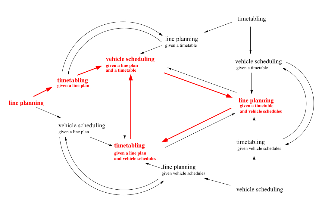
Figure 10 depicts a graph (called Eigenmodel) which illustrates finding a starting solution as well as the iteration steps (red). Notice that it contains more nodes than the ones referring to the algorithms mentioned before. In particular, each path through the Eigenmodel corresponds to solving a sequence of suproblems and hence to a heuristic. The name Eigenmodel refers to the own (=eigen) subproblems which form the nodes of the depicted graph. Eigenmodels have been introduced in [12], and analyzed, e.g., in [8, 14].
In the examples presented, a scalar-valued objective function is associated with each subproblem resulting in multiple and conflicting objectives. As a result, a vector-valued objective function is related to the AiO problem but is ignored by the BCD heuristic that solves the single objective optimization problem at every stage. In this study we recognize the existence of an AiO vector-valued function that is carried by every subproblem at every stage. In other words, we deal with AiO multiobjective optimization problems (MOPs) that remain multiobjective at every stage. MOPs lend themselves to decomposition into multiobjective (or single objective) subproblems whose solutions shall provide the efficient solutions to the original MOPs. In the public transportation example one might follow several objectives: the costs of the public transport system should be minimized. At the same time, the traveling time for passengers as well as the carbon emission should be minimized.
The standard single objective BCD relies on a well-established algorithm with a proof of convergence [1] for continuous optimization problems. The contribution of this preliminary study is the formulation of the BCD for the biobjective two-stage case with some supporting theory and implementation variants. The latter include approximation algorithms and evolutionary heuristics.
4.7.2 Block coordinate descent algorithm for two criteria and two blocks
Consider the following biobjective unconstrained optimization problem with two blocks:
| (29) | |||
where , , and for are the two scalar coordinate directions, also referred to as blocks of one or more variables in the general block coordinate descent method. Let
-
denote the efficient set of (29)
-
denote the efficient set in iteration for block
-
denote the efficient set at the completion of iteration
-
denote the efficient set at the completion of N iterations
-
denote the operator of extracting the efficient points from an arbitrary set S
4.7.2.1 Algorithm: Biobjective Block Coordinate Descent (BBCD)
-
1.
Initialization: starting point (not necessarily an efficient starting solution), ,
-
2.
Iteration :
Set
-
3.
If stop, set , otherwise set and return to step 2.
To understand the properties of the proposed BBCD algorithm, the extension of block coordinate descent to the biobjective case, we seek to answer the following research questions. Let be the number of iterations of the BBCD algorithm ( can be assumed finite or infinite).
-
1.
Under which conditions does the set contain only efficient solutions, i.e., ?
-
2.
Under which conditions are all efficient solutions found, i.e., ?
-
3.
How big is , or in other words, what is the number of iterations needed to achieve the two goals above?
4.7.2.2 Auxiliary background
The following notation is used: a vector-valued function , scalar-valued function , level set , and level curve .
We also define the coordinate lines (hyperplanes) passing through a point for : , i.e. represents the coordinate line in the -direction.
Theorem 1 shows how level sets and curves can be used to characterize the efficient solutions of an unconstrained -objective optimization problem. Figure 11 depicts two level curves of two hypothetical objective functions indicating that a point is not efficient.
Theorem 1.
[6] Let and define . Then is efficient if and only if
| (30) |
A curve in is said to be smooth provided for every point on this curve there exists a neighborhood on which this curve is a graph of a differentiable function. In the following we assume differentiable and that is a smooth curve in , and therefore .
4.7.2.3 Conjectures with proof outlines
The first research question asks whether all solutions found by the BBCD are efficient, i.e., . In the following it is assumed that the functions are convex and differentiable.
Proof sketch for : Assume and . In particular, where is the number of iterations of the BBCD. According to Theorem 1, an efficient point satisfies (30). Since is not efficient, the intersection of the level sets and has a nonempty interior. Two cases of this intersection are shown in Figures 11 and 12.
In Case 1 depicted in Figure 11, we observe that the search into one of the search directions leads into the area containing solutions that improve both and , hence . In the scenario shown in Figure 11 the BBCD searches into the direction first. We note that in this case, remains an efficient solution in the search along as it cannot be dominated by other solutions encountered along (if there are any). (Also the search along yielded at least in the last iteration as . Once the BBCD searches in direction , solutions in the interior of are encountered. Since for any such solution we have a contradiction to . Similarly, such a solution would be encountered immediately if intersects the interior of .
In Case 2 depicted in Figure 12, the interior of and do not intersect for . Here, we know that, starting from , we can find efficient solutions along either or ( in the scenario shown in Figure 12). (Otherwise would be efficient as the level sets do not intersect). Moving at least some way in a direction that improves an objective ( in Figure 12) would yield other efficient solutions such that and do not dominate each other.
The point is shown in Figure 13 together with the level sets of where we have and .
The search along the other block from point will move towards and into the intersection as decreases and increases. We have for any solution . If itself is not efficient as there exists another constructed by the BBCD with , then we also have . This is a contradiction to .
The second research questions investigates whether all efficient solutions can be found by the BBCD. To address the question whether , the objective functions are assumed to be strictly convex (to avoid weakly efficient solutions). For the inclusion of interest, the differentiability is required to avoid stalling as happens in the following example (31) where the BBCD is unable to identify the complete .
| (31) | |||
In this example, the efficient set is .
Proof idea for : Start with an efficient solution in , and then demonstrate that the search will always expand outwards along connected efficient solutions until the lexicographic solutions are reached (and hence everything in between). This argument should work as the efficient set is connected for convex differentiable multiobjective optimization problems [11].
The third research question addresses the number of required iterations, i.e,. what is equal to? A first exploration of this question suggests the following observations. Firstly, we observe that in the case of a simple quadratic problem. Secondly, based on a nonlinear and convex example problem where is unbounded, an infinite number of iterations is required.
4.7.2.4 Ongoing and future work
The initial investigation presented in this section proposed the BBCD for a problem with two variables, where two of the research questions (the inclusion and the number of iterations) remain open. This theory needs to be further extended to the case of coordinate directions , or blocks of variables , as well as objectives.
We recognize that the block coordinate descent is a powerful heuristic tool to solve large-scale practical optimization problems. Further into the future, the proposed BBCD could be similarly applied as a heuristic for solving biobjective (mixed) integer linear programs. In order to find the most effective implementation in terms of a budget on computational resources or time, the analysis could be performed in two directions. First, the time to solve AiO problems shall be compared to the time to solve them with the BBCD. Second, working only with the BBCD, the time spent on balancing between solving individual subproblems and exchanging information between them needs to be analyzed.
4.7.3 Multiobjective Evolutionary Algorithms
As alluded to above, the block coordinate descent approach is employed in various applications of optimization such as transportation systems [17], wireless communication networks [18], signal processing [13], multiclass classification [2], and others. We aim to highlight through runtime analysis the benefit of incorporating the block coordinate approach into evolutionary multiobjective algorithms. We employ state-of-the-art algorithms such as the Global Simple Evolutionary Multiobjective Optimizer (GSEMO) [7] and the Nondominated Sorting Genetic Algorithm II (NSGA-II) [3].
We plan to use problems that we understand and analyze the runtime for GSEMO/NSGA-II when incorporating the block coordinate approach. Our aim is to provide an example where we can prove that the block coordinate descent incorporated into these evolutionary algorithms leads to an asymptotic speed up of the optimization process.
4.7.3.1 Algorithms with different levels of complexity
We consider how to implement the algorithm using three different “complexity" algorithms:
-
At each iteration, choose only one solution to continue
-
At each iteration, find all the locally Pareto optimal solutions and continue expanding this set (similar to the Pareto Local Search)
-
At each iteration, find only solutions to continue with, using something analogous to the ‘uncrowded hypervolume’ method.
We will compare with Pareto Local Search and multiobjective Branch-and-Bound algorithms to obtain or reuse results on how to continually expand a set to approximate a Pareto set. It might be possible to interpret the three different choices of implementation as budgets or relatable to budgets.
4.7.3.2 Candidate Problems
We consider the following problem candidates:
Possibilities for allocating budgets may be:
-
Computing the whole set of Pareto optimal solutions for a fixed set of search points
-
Allocating budgets for solving the different subproblems.
4.7.3.3 Runtime Analysis for Block Coordinate MOEAs
We now define a problem where we hope to show the benefit of incorporating the block coordinate approach. We consider a bi-objective version of the wCLOBl,k (concatenated LeadingOnes with blocks and weights) problem [5].
Our aim is to show a lower bound for the standard GSEMO (see Algorithm 3) and an upper bound for BC-GSEMO (see Algorithm 4), where the lower bound is lower than the upper bound. This would prove a clear advantage of BC-GSEMO over GSEMO for the problems considered. Let where is the ith block of the bitstring of length .
We define
as the number of leading positions where agrees with a given string .
Let and , where is an appropriate constant.
We consider the biobjective problem given as
We consider optimization using the classical GSEMO algorithm (see Algorithm 3) as well as a block coordinate variant called BC-GSEMO (see Algorithm 4). The algorithm optimizes the blocks sequentially and terminates if the optimization part for the current block does not change the population, i.e., there is no change to the population when executing the repeat loop.
To apply the block coordinate mutation to block , we flip each bit of independently of the others with probability . For the local variant called the Block coordinate SEMO (BC-SEMO), one randomly chosen bit is flipped in the chosen block .
We consider different budgets of , e.g.,
-
(slow parallel progress, good runtime bounds s)
-
, appropriate large constant (optimizes block for each individual in the population if population size is constant)
-
, appropriate large constant (optimizes block for each individual in the population).
Note that a careful consideration is required for different choices of , which is potentially dependent on the current population size.
Let be the set of all search points for which where for all . Note that for each search point , there is at least one search point in that strongly dominates . Hence, those search points are not Pareto optimal.
For each , we have
Furthermore, let be two search points with . Then we have and . This implies that each search point is Pareto optimal and the Pareto front is given by .
We provided this problem and the algorithmic setting. It remains to show that BC-GSEMO outperforms GSEMO on the problem by providing upper and lower bounds for the algorithms that show the conjectured difference in performance. During the seminar, we worked on proving a conjecture, and believe we may have a result showing an asymptotic advantage to BC-GSEMO based on the application of modern drift theory. The result follows from differences in the evolving population size in the optimization phases of each algorithm, and different interactions between solutions, with BC-GSEMO suffering from less negative drift.
Our goal is also to complement the theoretical analysis with an experimental study on problem instances of realistic size and examine the performance of the two algorithms in terms of the dependence of the input size, and when different types of budget are imposed.
References
- [1] D.P. Bertsekas. Nonlinear Programming. Athena Scientfic, Belmont, Massachusetts, 2016.
- [2] Mathieu Blondel, Kazuhiro Seki, and Kuniaki Uehara. Block coordinate descent algorithms for large-scale sparse multiclass classification. Machine Learning, 93(1):31–52, 2013.
- [3] Kalyanmoy Deb, Samir Agrawal, Amrit Pratap, and T. Meyarivan. A fast and elitist multiobjective genetic algorithm: NSGA-II. IEEE Transactions on Evolutionary Computation, 6(2):182–197, 2002.
- [4] T. Dietz, K. Klamroth, K. Kraus, S. Ruzika, L. Schäfer, B. Schulze, M. Stiglmayr, and M. M. Wiecek. Introducing multiobjective complex systems. European Journal of Operational Research, 280:581–596, 2020.
- [5] Benjamin Doerr, Dirk Sudholt, and Carsten Witt. When do evolutionary algorithms optimize separable functions in parallel? In FOGA, pages 51–64. ACM, 2013.
- [6] M. Ehrgott. Multicriteria Optimization. Springer, second edition, 2005.
- [7] Oliver Giel. Expected runtimes of a simple multi-objective evolutionary algorithm. In IEEE Congress on Evolutionary Computation, pages 1918–1925. IEEE, 2003.
- [8] S. Jäger and A. Schöbel. The blockwise coordinate descent method for integer programs. Mathematical Methods of Operations Research, 91:357–381, 2020.
- [9] K. Klamroth, S. Mostaghim, B. Naujoks, S. Poles, R. Purshouse, G. Rudolph, S. Ruzika, S. Sayin, M.M. Wiecek, and X. Yao. Multiobjective optimization for interwoven systems. Journal of Multi-Criteria Decision Analysis, 24:71–81, 2017.
- [10] Per Kristian Lehre. Runtime analysis of competitive co-evolutionary algorithms for maximin optimisation of a bilinear function. In GECCO, pages 1408–1416. ACM, 2022.
- [11] K. Miettinen. Nonlinear Multiobjective Optimization. Kluwer Academic Publishers, Boston, 1999.
- [12] A. Schöbel. An eigenmodel for iterative line planning, timetabling and vehicle scheduling in public transportation. Transportation Research C, 74:348–365, 2017.
- [13] Dongyuan Shi, Bhan Lam, Woon-Seng Gan, and Shulin Wen. Block coordinate descent based algorithm for computational complexity reduction in multichannel active noise control system. Mechanical Systems and Signal Processing, 151:107346, 2021.
- [14] P. Schiewe and A. Schöbel. Integrated optimization of sequential processes: General analysis and application to public transport. EURO Journal on Transportation and Logistics, 11:100073, 2022.
- [15] M.M. Wiecek and P. de Castro. Developing decomposition-coordination techniques for many-objective tradeoff analysis. In S. Greco, V. Mousseau, J. Stefanowski, and C. Zopounidis, editors, Intelligent Decision Support Systems – Combining Operations Research and Artificial Intelligence, Springer Series on MCDM, pages 307–329. Springer, 2022.
- [16] Richard A. Watson, Gregory Hornby, and Jordan B. Pollack. Modeling building-block interdependency. In PPSN, volume 1498 of Lecture Notes in Computer Science, pages 97–108. Springer, 1998.
- [17] Zewen Wang, Kai Zhang, Xinyuan Chen, Meng Wang, Renwei Liu, and Zhiyuan Liu. An improved parallel block coordinate descent method for the distributed computing of traffic assignment problem. Transportmetrica A: Transport Science, 18(3):1376–1400, 2022.
- [18] Qingqing Wu, Yong Zeng, and Rui Zhang. Joint trajectory and communication design for multi-uav enabled wireless networks. IEEE Trans. Wirel. Commun., 17(3):2109–2121, 2018.
4.8 Exploring correlations in multi-objective optimization
Tea Tusar (Jozef Stefan Institute – Ljubljana, SI), Dimo Brockhoff (INRIA Saclay – Palaiseau, FR), Jonathan Fieldsend (University of Exeter, GB), Boris Naujoks (TH Köln, DE), Alma Rahat (Swansea University, GB), Vanessa Volz (modl.ai – Copenhagen, DK), Hao Wang (Leiden University, NL), Kaifeng Yang (Univ. of Applied Sciences – Hagenberg, AT)
License: Creative Commons BY 4.0 International license © Tea Tusar, Dimo Brockhoff, Jonathan Fieldsend, Boris Naujoks, Alma Rahat, Vanessa Volz, Hao Wang, and Kaifeng Yang
4.8.1 Introduction
A frequent assumption in evolutionary computation is that all function evaluations take the same amount of time. However, this rarely holds for real-world optimization problems, especially those that rely on simulations for evaluating solutions. There, the evaluation time can differ for different objectives as well as for different solutions.
The case where evaluation time depends on objectives has already been explored in a previous Dagstuhl Seminar [7]. This typically occurs in problems where some objectives can be computed with a closed-form expression while others require lengthy simulations. Various strategies for handling objectives with heterogeneous evaluation times are reviewed in [1].
During this seminar, we focused on the second case, in which the evaluation time depends on solutions. Specifically, we wanted to explore whether the correlation between objectives and their evaluation times can be modeled and exploited to save expensive function evaluations.
4.8.2 Motivation from real-world applications
In some real-world problems, the relation between solution properties and evaluation times is rather straightforward. For example, in the tunnel alignment problem [9], where a solution represents a tunnel trajectory, the computational expense of assessing tunnel objectives and constraints is proportional to the length of the tunnel – a longer tunnel will generally take longer to evaluate. Similarly holds for neural architecture search [3], where a solution defines the architecture of a neural network whose training time is strongly positively correlated with its size.
However, there are also other kinds of real-world problems where such a relation is hard to find. Consider the airfoil optimization problem [11], where computational fluid dynamics is used in solution evaluation, and the electrical motor design problem [13], which relies on electromagnetic field simulations. In both cases, evaluation times vary among solutions, but a clear correlation between solution characteristics and evaluation duration has not been discovered.
Another source of solution-dependent evaluation times is the presence of hidden constraints. For instance, the MarioGAN optimization problem [14] involves generating Mario game levels, which are assessed through playthrough simulations with artificial intelligence players. If a generated level cannot be solved (that is, Mario cannot reach the level end), the simulation would continue endlessly unless terminated. The distance in the search space between feasible solutions that are relatively quick to evaluate and infeasible solutions whose evaluation takes a long time can be very small in such cases.
These examples show that the correlation between objective quality and its evaluation time depends on the problem and the solutions. We can model it by considering the evaluation time as an additional independent objective to be minimized.
4.8.3 Visualization of correlations
We use search space visualizations to gain a better understanding of the correlations between objectives. The correlation for each pair of objectives is estimated in different regions of the search space using the Pearson correlation coefficient for a small (local) sample of the search space. The Pearson correlation coefficient measures the linear correlation between two samples’ objectives and takes a value between (perfect linear anti-correlation) and (perfect linear correlation). A value implies that there is no linear dependency between the objectives. The Pearson correlation coefficient is invariant when the two objectives are shifted and/or scaled.
4.8.3.1 Experimental setup
For demonstration purposes, we choose some continuous test problems with 2-D search spaces that are straightforward to visualize. They have either two, three or five objectives and various characteristics (more details below). We assume minimization of their objectives.
The 2-D problem search space is discretized into a grid of points. For each grid point , the correlation between two objectives is computed with the Pearson correlation coefficient as follows. First, equidistant points are created on the circle with radius centered at with one point placed at position , see Figure 14. Next, the points are evaluated, i.e. objective values are computed for each of them. Finally, the correlation between each pair of objectives at is estimated with the corresponding Pearson correlation coefficient for the set of points. Note that the points could have been constructed also in some other way. We opted for this deterministic approach to minimize the disturbances caused by a stochastic choice of point placement. In all experiments, the number of points was set to 100.
4.8.3.2 Problems with two objectives
First, we wish to explore the simplest case of two objectives. For this, we select six bi-objective problems from the bbob-biobj suite of benchmark problems [2]. They are constructed by combining two single-objective functions from the bbob suite [8]. Figure 15 shows the visualization of correlations between the two objectives for each of the six problems.
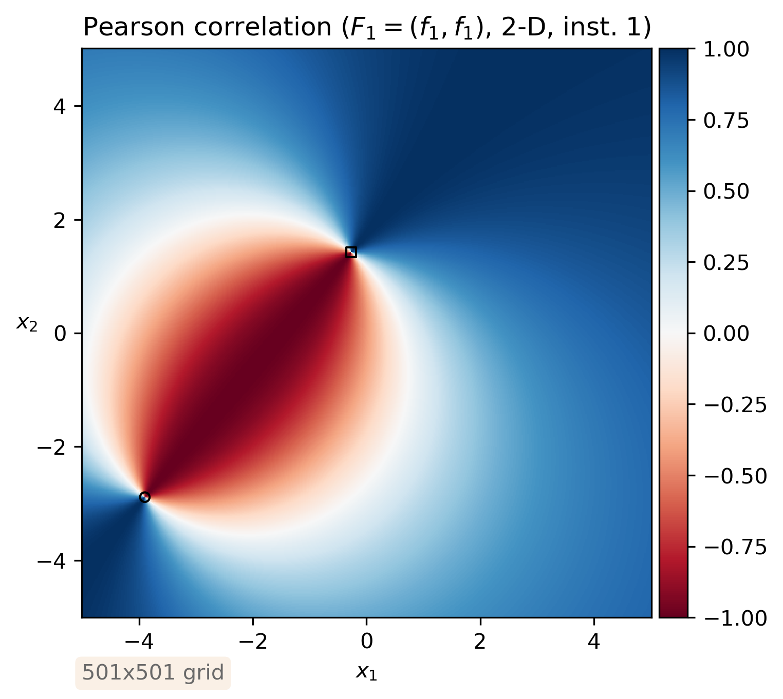
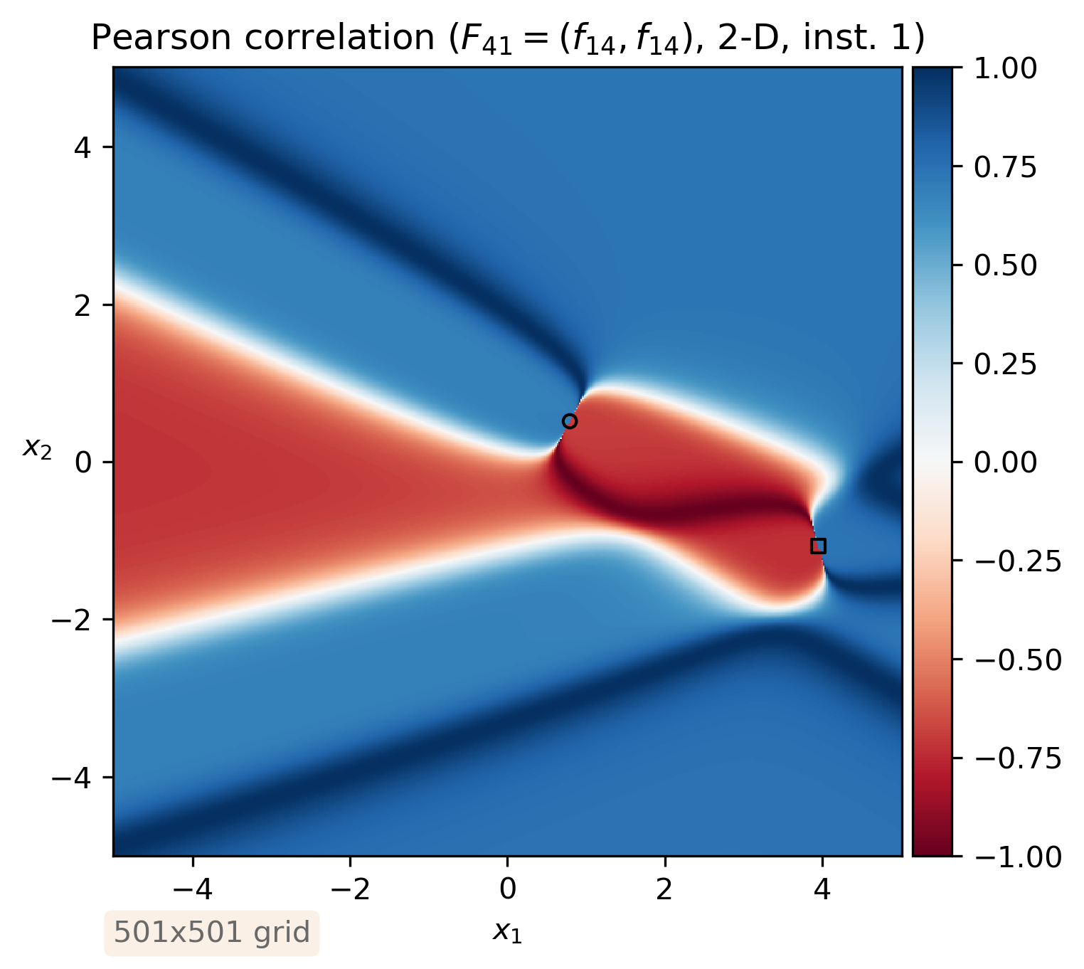
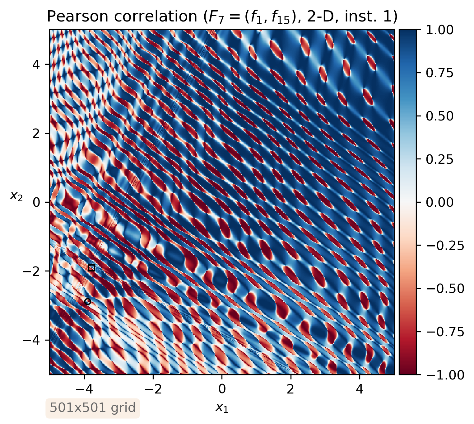
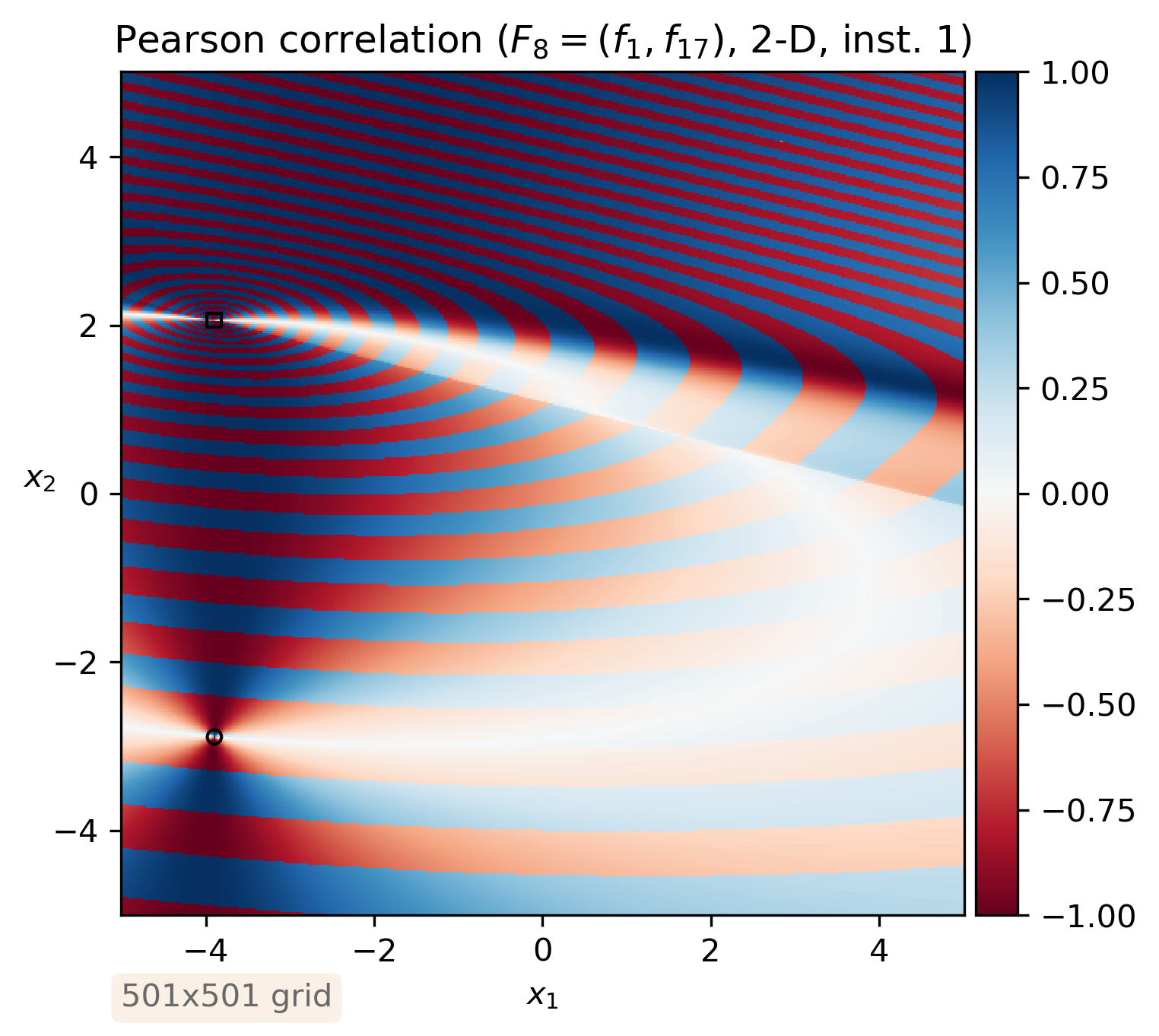
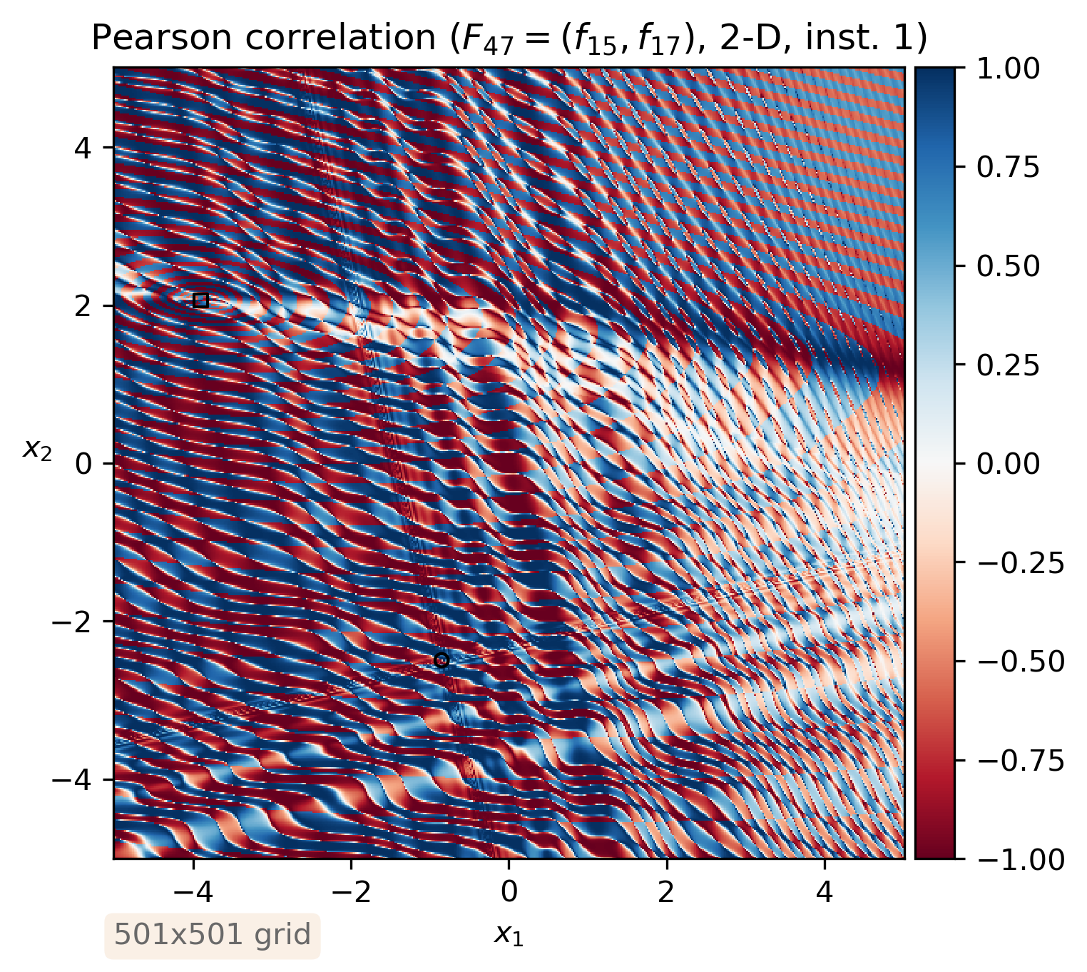
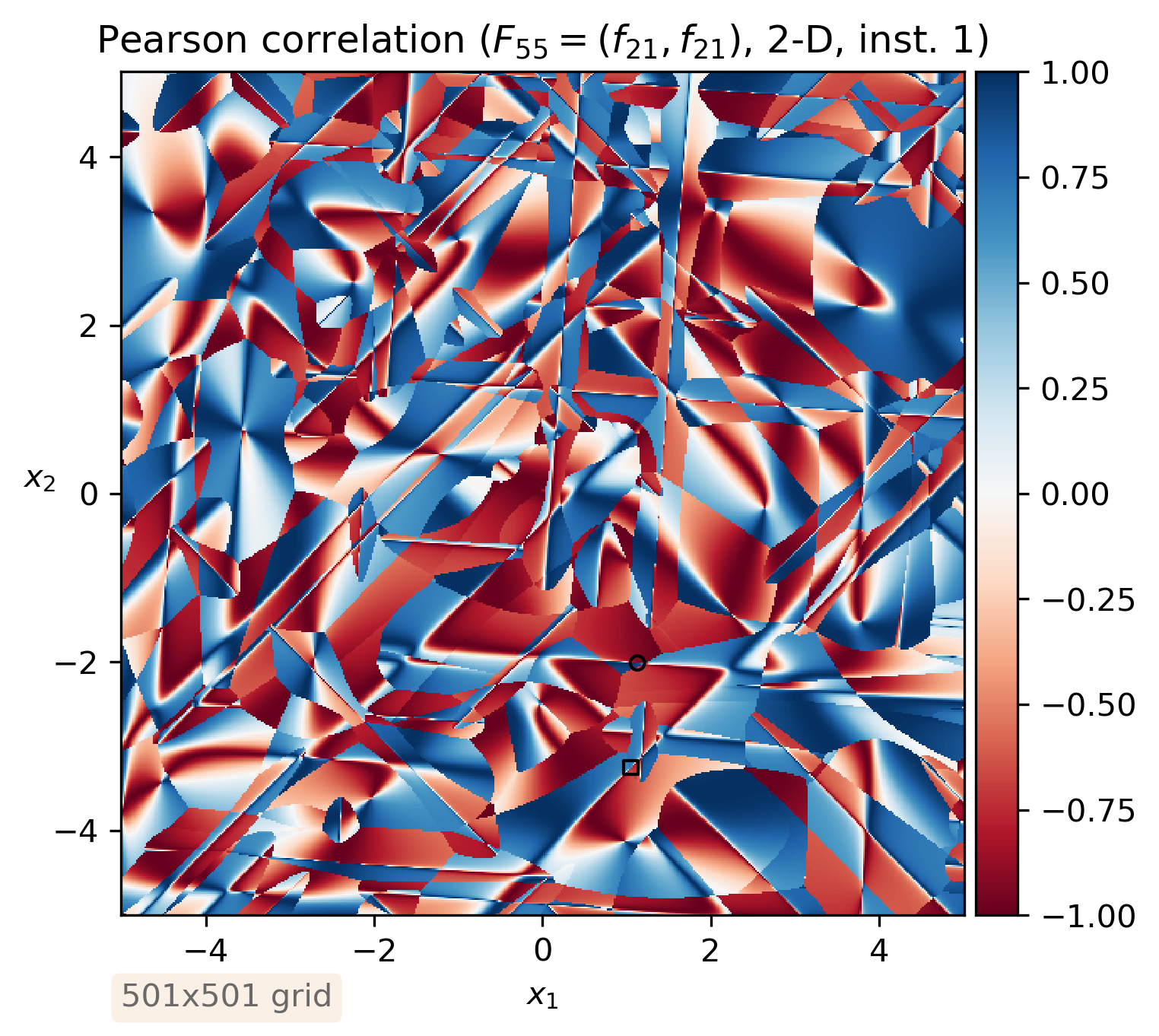
The double sphere problem , where is the bbob sphere function, is a unimodal problem with a known Pareto set – the line segment connecting the two single-objective optima. We can see from the correlation plot in Figure 15(a) the expected outcome – close to the Pareto set, the objectives are anti-correlated (red hues), while further away they are correlated (blue hues).
In the problem , both objectives are unimodal as well, but they correspond to the bbob sum of different powers function , which is non-separable and ill-conditioned. Figure 15(b) shows that in this case, the objectives are anti-correlated also far away from the Pareto set.
The next two problems are a combination of a unimodal objective (the bbob sphere function ) and a highly multimodal one. In the problem , this is the bbob Rastrigin function , while in the problem , it is the bbob Schaffer F7 function with condition number 10. In both instances, visualized in Figures 15(c) and 15(d), the resulting bi-objective problems have multiple disconnected regions of the search space where the objectives are anti-correlated.
Finally, in the last two selected problems, both objectives are highly multimodal. The problem combines the bbob Rastrigin function with the bbob Schaffer F7 function with condition number 10 and the problem two bbob Gallagher’s Gaussian functions with 101 median peaks. We can see from the correlation plots in Figures 15(e) and 15(f) the high number of disconnected regions of anti-correlated objectives.
These examples challenge some of our preexisting notions about the correlation between objectives. In particular, they show that it is closely connected to the problem multimodality – understandably, given that the correlation between two objectives equals at any locally optimal set. In fact, the notion of a globally (i.e., Pareto) optimal set is inconsequential for correlation values. It is therefore rather meaningless to discuss correlations between objectives without taking into account their multimodality. We also see that the Pearson correlation coefficient values are themselves positively correlated with the length of the normalized bi-objective gradient as defined in [10] and visualized in [2].
4.8.3.3 Problems with three objectives
The Pearson correlation coefficient is defined only for two objectives. When the objectives are three (or more), we can compute all their pairwise correlations. We wish to visualize their minimal values to emphasize parts of the search space with the highest anti-correlation as they are locally optimal.
Exemplary three-objective problems are again constructed by combining bbob functions – now three. This time, we chose the triple sphere problem, the sphere-Rastrigin-Schaffer problem and the triple Gallagher problem. See Figure 16 for their visualizations. For each problem we show on the left hand side the pairwise correlations for objectives 1 and 2, objectives 1 and 3 and objectives 2 and 3 as well as their mean. On the right hand side, their minimum is presented.
The Pareto set of the triple sphere problem is the triangle spanned by the three single-objective optima. From Figure 16(a) we see that its minimal pairwise Pearson correlation coefficient equals only at the edges of this triangle, not in its interior. This shows that, unlike in the bi-objective case, one cannot rely on pairwise correlations alone to infer local optimality of a solution in case of more than two objectives. A procedure similar to the one from [12] should be tried to amend this issue.
4.8.3.4 Problems with five objectives
We next consider a couple of planar problems with five objectives, using the distance-based multi-objective point problem (DBMOPP) generator [5]. This generator allows us to create problem instances which natively live in 2-D (or map to 2-D), which can have an arbitrary number of objectives and can exhibit a range of other problem properties.
We first generate a box-constrained instance with a single spatially contiguous Pareto set (shown in red in Figure 17(a)) and seven other regions which generate local fronts of the same shape, but which are dominated (shown in green in Figure 17(a)). Figure 17(b) shows the corresponding dominance landscape [4]. Black regions in this figure show locations which are not dominated by any immediate neighbor (dominance neutral regions). Gray regions in contrast denote locations which have at least one dominating neighbor, but where all point-based dominance hill-climbs (by moving to an adjacent dominating neighbor) lead to the same dominance neutral region – different shades of gray are used to distinguish these different basins. White regions signify where point-based dominance hill-climbs lead to multiple different dominance neutral regions (effectively multi-objective saddle-points), depending on which chain of dominating neighbors one follows. Figure 17(c) shows the dominance ratio [6] landscape for the problem instance. In this plot, the value at a location denotes the proportion of the entire domain which weakly dominates it (i.e. dominates or is equal to it). That is, a value of 0.0 will indicate a location is Pareto optimal, whereas a value of 0.2 indicates that 20% of the domain relates to locations with equal or better performance on all criteria. Pearson correlation plots are shown in Figures 17(d)–17(f). For this problem we can see the eight distinct local optima regions clearly in the Dominance ratio plot, with the induced dominance neutral plateaus between these regions additionally identifiable in the dominance landscape and correlation plots.
The second example shown in Figure 18(a) has a single spatially contiguous Pareto set region (red), 3 dominance resistance regions (blue), 3 local fronts regions (green) and 30% of the decision space is designed as being flat under the objectives (cyan). The corresponding dominance landscape is shown in 18(b), and the dominance ratio landscape in 18(c). Pearson correlation plots are shown in Figures 18(d)–18(f). The impact of the flat objective regions is clear across the plots, and all views of the landscape are considerably more cluttered due to the interactions of the various problem features.
4.8.4 Conclusions
We recognized that evaluation times can differ among solutions of expensive real-world problems. We were therefore interested in exploring whether the correlation between objectives and their evaluation times can be used to save time-consuming function evaluations. A deeper look into the properties of some real-world applications has shown that a general model for such a correlation is hard to find. Therefore, the evaluation time was regarded as an additional objective to be minimized.
Next, we researched the correlation between objectives, estimating it with the Pearson correlation coefficient. To gain a better understanding of the distribution of its values in the search space, we visualized them for a number of test problems with two variables and two, three and five objectives. The visualizations have shown that some of our intuition about the correlation between objectives was wrong. For example, we could find unimodal problems with anti-correlated objectives not only close to the Pareto set, but also far away from it. Visualizations of multimodal problems have proven that many distinct anti-correlated regions can be located throughout the search space, surrounded by regions with correlated objectives. In fact, the visualizations have demonstrated that correlation is closely tied to the problem multimodality and has a nonlinear monotonous relation with the length of the bi-objective gradient. Finally, while pairwise anti-correlations between objectives correspond to the locally optimal solutions for problems with two objectives, this is no longer the case when the number of objectives is three or more.
References
- [1] Richard Allmendinger and Joshua D. Knowles. Heterogeneous objectives: State-of-the-art and future research. CoRR, abs/2103.15546, 2021.
- [2] Dimo Brockhoff, Anne Auger, Nikolaus Hansen, and Tea Tušar. Using well-understood single-objective functions in multiobjective black-box optimization test suites. Evolutionary Computation, 30(2):165–193, 2022.
- [3] Thomas Elsken, Jan Hendrik Metzen, and Frank Hutter. Neural architecture search: A survey. Journal of Machine Learning Research, 20(55):1–21, 2019.
- [4] Jonathan E. Fieldsend, Tinkle Chugh, Richard Allmendinger, and Kaisa Miettinen. A feature rich distance-based many-objective visualisable test problem generator. In Proceedings of the Genetic and Evolutionary Computation Conference, GECCO ’19, page 541–549, New York, NY, USA, 2019. Association for Computing Machinery.
- [5] Jonathan E. Fieldsend, Tinkle Chugh, Richard Allmendinger, and Kaisa Miettinen. A visualizable test problem generator for many-objective optimization. IEEE Transactions on Evolutionary Computation, 26(1):1–11, 2022.
- [6] Carlos Manuel Mira da Fonseca. Multiobjective genetic algorithms with application to control engineering problems. PhD thesis, University of Sheffield, 1995.
- [7] Salvatore Greco, Kathrin Klamroth, Joshua D. Knowles, and Günter Rudolph. Understanding complexity in multiobjective optimization (Dagstuhl Seminar 15031). Dagstuhl Reports, 5(1):96–163, 2015.
- [8] Nikolaus Hansen, Steffen Finck, Raymond Ros, and Anne Auger. Real-parameter black-box optimization benchmarking 2009: Noiseless functions definitions. Research Report RR-6829, INRIA, 2009.
- [9] Miha Hafner, David Rajšter, Marko Žibert, Tea Tušar, Bernard Ženko, Martin Žnidaršič, Flavio Fuart, and Daniel Vladušič. Artificial intelligence support for tunnel design in urban areas. In Tunnels and Underground Cities: Engineering and Innovation meet Archaeology, Architecture and Art- Proceedings of the WTC 2019 ITA-AITES World Tunnel Congress, pages 2196–2205, 2019.
- [10] Pascal Kerschke and Christian Grimme. An expedition to multimodal multi-objective optimization landscapes. In Evolutionary Multi-Criterion Optimization – 9th International Conference, EMO 2017, Münster, Germany, March 19-22, 2017, Proceedings, volume 10173 of Lecture Notes in Computer Science, pages 329–343. Springer, 2017.
- [11] Boris Naujoks, Werner Haase, Jörg Ziegenhirt, and Thomas Bäck. Multi objective airfoil design using single parent populations. In GECCO 2002: Proceedings of the Genetic and Evolutionary Computation Conference, New York, USA, 9-13 July 2002, pages 1156–1163. Morgan Kaufmann, 2002.
- [12] Lennart Schäpermeier, Christian Grimme, and Pascal Kerschke. To boldly show what no one has seen before: A dashboard for visualizing multi-objective landscapes. In Evolutionary Multi-Criterion Optimization – 11th International Conference, EMO 2021, Shenzhen, China, March 28-31, 2021, Proceedings, volume 12654 of Lecture Notes in Computer Science, pages 632–644. Springer, 2021.
- [13] Tea Tušar, Peter Korošec, and Bogdan Filipič. A multi-step evaluation process in electric motor design. In Slovenian Conference on Artificial Intelligence, Proceedings of the 26rd International Multiconference Information Society – IS 2023, volume A, pages 48–51. Jožef Stefan Institute, 2023.
- [14] Vanessa Volz, Boris Naujoks, Pascal Kerschke, and Tea Tušar. Single- and multi-objective game-benchmark for evolutionary algorithms. In Proceedings of the Genetic and Evolutionary Computation Conference, GECCO 2019, Prague, Czech Republic, July 13-17, 2019, pages 647–655. ACM, 2019.
5 Seminar Schedule
Monday, September 4, 2023
- 09:00–10:30
-
Welcome Session
-
•
Welcome and introduction
-
•
Short presentation of all participants
-
•
-
Coffee Break
- 11:00–12:00
-
Seminar Overview
-
•
Seminar scope
-
•
Offers-and-needs market
-
•
-
Lunch
- 14:00–15:30
-
Modelling to Address Budget Constraints
-
•
Juliane Mueller: Surrogate model guided optimization of expensive black-box multiobjective problems
-
•
Andrea Raith: Problem decomposition in biobjective optimization
-
•
-
Coffee Break
- 16:00–16:30
-
Working Group Formation
- 16:30–18:00
-
Working Groups
-
Dinner
Tuesday, September 5, 2023
- 09:00–09:30
-
Reporting from Small Working Groups Chair: Matthias Ehrgott
- 09:30–10:30
-
Small Working Groups
-
Coffee Break
- 11:00–12:00
-
Heuristic Optimization and Human Involvement Chair: Jürgen Branke
-
•
Thomas Bäck: How to help end users when the budget is limited?
-
•
Robin Purshouse: Towards decision analytic workflows for real-world problems: Simulation model calibration and multi-objective optimization on a shared evaluation budget
-
•
Benjamin Doerr: Runtime analysis for the NSGA-II
-
•
Kaisa Miettinen: Perspectives to dealing with computationally expensive multiobjective optimization problems
-
•
-
Lunch
- 14:00–15:30
-
Small Working Groups
-
Coffee Break
- 16:00–17:00
-
Small Working Groups
- 17:00–18:00
-
Reporting from Small Working Groups and General Discussion
-
Dinner
Wednesday, September 6, 2023
- 09:00–10:30
-
Small Working Groups
-
Coffee Break
- 11:00–12:00
-
Approximation and Exact Methods Chair: Karl-Heinz Küfer
-
•
Kathrin Klamroth: Objective space methods: Pareto front approximations on a budget
-
•
Michael Stiglmayr: Multi-objective branch-and-bound on a budget
-
•
Frank Neumann: Fast Pareto optimization using sliding window selection
-
•
Alma Rahat: Efficient approximation of expected hypervolume improvement using Gauss-Hermite quadrature
-
•
- 12:00-12:15
-
Group Photo Outside
-
Lunch
- 13:30–15:30
-
Hiking Trip
-
Coffee Break
- 16:00–18:00
-
Small Working Groups
-
Dinner
Thursday, September 7, 2023
- 09:00–10:00
-
Reporting from Small Working Groups Chair: Kaisa Miettinen
-
Coffee Break
- 10:30–12:00
-
Small Working Groups
-
Lunch
- 14:00–15:30
-
Small Working Groups
-
Coffee Break
- 16:00–16:30
-
Graphical and probabilistic approaches Chair: Boris Naujoks
-
•
Ralph Steuer: A visualization-aided approach for solving tri-criterion portfolio problems
-
•
Hao Wang and Kaifeng Yang: Probability of “improvement” in multi-objective Bayesian optimization
-
•
- 16:30–17:00
-
Announcements
- 17:00–18:00
-
Joint session with DS22362
-
Dinner
- 20:00–23:00
-
Informal Get Together (BYOB, meet in the cafeteria)
Friday, September 8, 2023
- 09:00–10:30
-
Final Reporting from Working Groups
-
Coffee Break
- 11:00–12:00
-
Closing Session
6 Topics of interest for participants for next Dagstuhl Seminar
In the closing session on Friday, the participants reflected upon their experience and presented their ideas on a potential future seminar that would leverage the progress made during the current one. During this discussion, some topics appeared to center around “Artificial Intelligence (AI)”. A two-way perspective was suggested: AI for multiobjective optimization and multiobjective optimization for AI. Another suggestion was to focus on the “gap” between the industrial and the academic practice of multiobjective optimization. This suggestion was well-received by both industrial and academic participants of the seminar as the focus during the week was on a “budget” that might also mean decision maker’s limitations. Focusing on how the theoretical and methodological achievements on the academic front can be made more accessible to practitioners in industry may be a future direction to pursue. This direction will also possibly require placing more emphasis on modelling, handling the noise, errors and uncertainties in the process. The organizers will use these suggestions as the basis for their discussion about possible topics for the next edition of this seminar series and for the preparation of a proposal for a continuation of the series.
7 Changes in the seminar organization body
As part of a continuing effort to renew the organizing board of this series of Dagstuhl Seminars, Margaret Wiecek steps down from the team of organizers, a role that she has held for three terms of office. On behalf of all the participants of the seminar, Richard Allmendinger, Carlos Fonseca and Serpil Sayin would like to express appreciation to Margaret for her contributions and leadership that have been fundamental for the series success.
We are pleased to announce that our esteemed colleague and a multiple-times Dagstuhl attendee Susan Hunter has agreed to serve as a co-organizer for future editions of this Dagstuhl Seminar series on Multiobjective Optimization. We look forward to collaborating with her in the near future.
8 Participants
-
Thomas Bäck – Leiden University, NL
-
Mickaël Binois – INRIA – Sophia Antipolis, FR
-
Fritz Bökler – Universität Osnabrück, DE
-
Jürgen Branke – University of Warwick, GB
-
Dimo Brockhoff – INRIA Saclay – Palaiseau, FR
-
Tinkle Chugh – University of Exeter, GB
-
Kerstin Dächert – HTW Dresden, DE
-
Benjamin Doerr – Ecole Polytechnique – Palaiseau, FR
-
Matthias Ehrgott – Lancaster University, GB
-
Gabriele Eichfelder – TU Ilmenau, DE
-
Jonathan Fieldsend – University of Exeter, GB
-
Carlos M. Fonseca – University of Coimbra, PT
-
Susan R. Hunter – Purdue University, US
-
Ekhine Irurozki – Telecom Paris, FR
-
Hisao Ishibuchi – Southern Univ. of Science and Technology – Shenzen, CN
-
Andrzej Jaszkiewicz – Poznan University of Technology, PL
-
Pascal Kerschke – TU Dresden, DE
-
Kathrin Klamroth – Universität Wuppertal, DE
-
Joshua D. Knowles – Schlumberger Cambridge Research, GB
-
Karl Heinz Küfer – Fraunhofer ITWM – Kaiserslautern, DE
-
Arnaud Liefooghe – University of Lille, FR
-
Kaisa Miettinen – University of Jyväskylä, FI
-
Juliane Mueller – NREL – Golden, US
-
Boris Naujoks – TH Köln, DE
-
Aneta Neumann – University of Adelaide, AU
-
Frank Neumann – University of Adelaide, AU
-
Markus Olhofer – HONDA Research Institute Europe GmbH – Offenbach, DE
-
Luís Paquete – University of Coimbra, PT
-
Robin Purshouse – University of Sheffield, GB
-
Alma Rahat – Swansea University, GB
-
Andrea Raith – University of Auckland, NZ
-
Enrico Rigoni – ESTECO SpA – Trieste, IT
-
Stefan Ruzika – RPTU – Kaiserslautern, DE
-
Serpil Sayin – Koc University – Istanbul, TR
-
Anita Schöbel – Fraunhofer ITWM – Kaiserslautern, DE
-
Britta Schulze – Universität Wuppertal, DE
-
Ralph E. Steuer – University of Georgia, US
-
Michael Stiglmayr – Universität Wuppertal, DE
-
Tea Tusar – Jozef Stefan Institute – Ljubljana, SI
-
Daniel Vanderpooten – University Paris-Dauphine, FR
-
Vanessa Volz – modl.ai – Copenhagen, DK
-
Hao Wang – Leiden University, NL
-
Margaret M. Wiecek – Clemson University, US
-
Kaifeng Yang – Univ. of Applied Sciences – Hagenberg, AT
![[Uncaptioned image]](x3.jpg)