Triangulations in Geometry and Topology
Abstract
This report documents the program and the outcomes of Dagstuhl Seminar “Triangulations in Geometry and Topology” (24072). The seminar was held from February 12 to February 16, 2024, gathered 31 participants, and started with four introductory talks and an open problem session. Then the participants spread into small groups to work on open problems on diverse topics including reconfiguration of geometric shapes, geodesics on triangulated surfaces, distances in flip graphs, geometric cycles and algorithms in 3-manifold topology.
Keywords and phrases:
computational geometry, geometric topology, triangulationsSeminar:
February 11–16, 2024 – https://www.dagstuhl.de/240722012 ACM Subject Classification:
Human-centered computing Graph drawings ; Mathematics of computing Geometric topology ; Theory of computation Computational geometryCopyright and License:
![[Uncaptioned image]](x1.png) Except where otherwise noted, content of this report is licensed under a
Creative Commons BY 4.0 International license
Except where otherwise noted, content of this report is licensed under a
Creative Commons BY 4.0 International license
1 Executive Summary
Maike Buchin
Jean Cardinal
Arnaud de Mesmay
Jonathan Spreer
License: ![[Uncaptioned image]](x2.png) Creative Commons BY 4.0 International license © Maike Buchin, Jean Cardinal, Arnaud de Mesmay, and Jonathan Spreer
Creative Commons BY 4.0 International license © Maike Buchin, Jean Cardinal, Arnaud de Mesmay, and Jonathan Spreer
This seminar was a followup to the Dagstuhl Seminars “Applications of Topology to the Analysis of 1-Dimensional Objects” (17072), “Computation in Low-Dimensional Geometry and Topology” (19352), and “Computation and Reconfiguration in Low-Dimensional Topological Spaces” (22062). The common idea behind all of these seminars is to bring together researchers from different communities (such as computational geometry, graph drawing, or geometric topology) with a shared interest in low-dimensional objects (e.g., curves, embedded graphs, knots, or surfaces). The goal of this approach is to foster collaborative work and synergies: The mathematical study of low-dimensional objects has a rich and old history, but research into their algorithmic and combinatorial properties and the underlying computational questions is still young. This makes for a vibrant research situation, giving strong opportunities for interdisciplinary work involving our multiple communities.
The focus of this Dagstuhl Seminar was placed on triangulations: partitions of the plane into triangles, or, more generally, of a space into simplices, which are required to meet face-to-face. Triangulations are typically constrained to use a given set of points as vertices and are fundamental tools in many applications such as computer graphics or geographic information systems. Alternatively, a triangulation can be defined on a topological space as a simplicial complex together with a homeomorphism from this simplicial complex to the space. These triangulations play an important role in the study of metrics on surfaces and their moduli space. The multiple facets of triangulations make them an essential and ubiquitous object of study in the combinatorial, algorithmic, geometric and topological properties of low-dimensional spaces, and thus they constitute a fertile ground for collaborations.
The seminar started with a quick introduction of all the participants, and four keynote talks on different aspects of triangulations.
-
Lionel Pournin gave an overview of flip graphs and their combinatorial and algorithmic properties.
-
Saul Schleimer surveyed the use of triangulations in 3-manifold topology and the numerous computational challenges that arise from them.
-
Linda Kleist presented two snapshots on triangulations, first on the computational complexity of linearly embedding simplicial complexes, and then on some hamiltonicity properties of polytopes arising from flipping triangulations.
-
Mikkel Abrahamsen explained new hardness proofs for algorithmic problems related to packing, covering and partitioning simple polygons with unit squares.
We refer to the abstracts later in this report for more details on these contributions.
These keynote introductory talks were followed with an extended open problem session where we gathered a large collection of open problems. Some of these were circulated in advance of the meeting, many of them were new. The remainder of the week was spent working in small groups actively trying to make progress on the most popular open problems. We made extensive use of the tool “Coauthor,” designed by Erik Demaine (MIT). This allowed for a very efficient recording of the progress made in the different groups. Regular progress reports allowed participants to easily switch between groups during the week, or to start new groups, leading to a very dynamic working environment.
We now quickly survey the different problems that have been worked on during this very productive week:
-
Computational complexity of problems in 3-manifold topology. This group discussed computational complexity for important algorithmic problems from -manifold topology. Examples of problems include showing that a knot is ribbon, and testing -efficiency in a -manifold triangulation (lead: Eric Sedgwick).
-
Veering triangulations and the flip graph. This group studied the effect on flip distances of surface triangulations if a veering structure in the associated layered triangulation is (lead: Saul Schleimer).
-
Flip distances. This group investigated distances in the flip graphs of triangulated convex -gons or annuli, both theoretically and algorithmically (lead: Jonathan Spreer).
-
Hardness for simple polygons. The group considered NP-hard problems on polygons with holes, and how to show that these are also NP-hard on simple polygons. (lead: Lena Schlipf)
-
Catching balls on Curves. This group considered the problem of characterising curves for which there exist a strategy to catch a ball from any initial configuration. (lead: Maarten Löffler)
-
Computing geodesic paths using edge flips. This group investigated the FlipOut algorithm defined by Crane and Sharp to compute geodesics on intrinsic geometric triangulations and its possible variants. (lead: Hsien-Chih Chang)
-
Rendering a knot without self-intersections. This group focused on using topological data analysis techniques to produce instructive 3D models of link diagrams (lead: Clément Maria)
-
Shortest cycle separating objects from . This group investigated the complexity of, given a collection of objects, computing the shortest cycle separating objects from objects, and how it behaves with respect to the parameter . This was explored in the setting of the plane with obstacles and then planar graphs with obstacles, with an eye towards separating handles in graphs embedded on surfaces. (lead: Éric Colin de Verdière)
In summary, this Dagstuhl Seminar provided a very fruitful research environment, allowing participants from very different backgrounds to work together on important open problems. Survey feedback from the participants highlighted how much the emphasis on intensive work in small groups was appreciated. In several of the working groups, significant progress was made, and the results are currently prepared to be submitted for publication. As in the previous meetings, the excellent quality of the Dagstuhl infrastructure and the impeccable support of the Dagstuhl staff provided a seamless experience for all the participants. We are hopeful that this successful experience will lead to follow-up Dagstuhl Seminars on related topics.
2 Table of Contents
3 Overview of Talks
3.1 Packing, Covering and Partitioning Simple Polygons with Unit Squares
Mikkel Abrahamsen (University of Copenhagen, DK)
License: Creative Commons BY 4.0 International license © Mikkel Abrahamsen
Main reference: Mikkel Abrahamsen, Nichlas Langhoff Rasmussen: “Partitioning a Polygon Into Small Pieces”, CoRR, Vol. abs/2211.01359, 2022.
We show that packing axis-aligned unit squares into a simple polygon is NP-hard, even when is an orthogonal and orthogonally convex polygon with half-integer coordinates. It has been known since the early 80s that packing unit squares into a polygon with holes is NP-hard [Fowler, Paterson, Tanimoto, Inf. Process. Lett., 1981], but the version without holes was conjectured to be polynomial-time solvable more than two decades ago [Baur and Fekete, Algorithmica, 2001].
Our reduction relies on a new way of reducing from Planar-3SAT. Interestingly, our geometric realization of a planar formula is non-planar. Vertices become rows and edges become columns, with crossings being allowed. The planarity ensures that all endpoints of rows and columns are incident to the outer face of the resulting drawing. We can then construct a polygon following the outer face that realizes all the logic of the formula geometrically, without the need of any holes.
This new reduction technique proves to be general enough to also show hardness of two natural covering and partitioning problems, even when the input polygon is simple. We say that a polygon is small if is contained in a unit square. We prove that it is NP-hard to find a minimum number of small polygons whose union is (covering) and to find a minimum number of pairwise interior-disjoint small polygons whose union is (partitioning), when is an orthogonal simple polygon with half-integer coordinates. This is the first partitioning problem known to be NP-hard for polygons without holes, with the usual objective of minimizing the number of pieces.
We also describe a -approximation algorithm for the partitioning problem, and -approximation algorithms for several related problems.
3.2 2 Snapshots – Geometric Embedding of Complexes & Facet-Hamiltonian Cycles in Generalized Associahedra
Linda Kleist (TU Braunschweig, DE)
License: Creative Commons BY 4.0 International license © Linda Kleist
Joint work of: Part 1: Mikkel Abrahamsen and Tillmann Miltzow; Part 2: Jean Cardinal, Stefan Felsner, Robert Lauff
Main reference: Jean Cardinal, Stefan Felsner, Linda Kleist, Robert Lauff. Facet-Hamiltonian Cycles in Permutohedra and
Generalized Associahedra. (in preparation)
In this talk, we will consider two snapshots of triangulations in geometry and topology.
In the first part, we consider the decision problem of determining whether a given (abstract simplicial) -complex has a geometric embedding in . In particular, we consider the case and , i.e., a geometric embedding corresponds to a set of triangles in 3D, and show that this problem is complete for the Existential Theory of the Reals (ETR). As a matter of fact the result can be extended to all and . We note that ETR-hardness implies NP-hardness and that our work constitutes the first hardness result for the algorithmic problem of geometric embedding of (abstract simplicial) complexes. This complements recent breakthroughs for the computational complexity of piece-wise linear embeddability. This part is based on joint work with Mikkel Abrahamsen and Tillmann Miltzow.
In the second part, we investigate facet-Hamiltonian cycles of polytopes, i.e., cycles in the skeleton such that every facet of the polytope is visited exactly once. These cycles can be understood as shortest tours that guard the facets of a polytope. Among other polytopes, we consider associahedra of type A where the 1-skeletons correspond to the flip graphs of triangulations of points in convex position. The skeletons of their generalizations, known as associahedra of type B/C and D, also allow for models involving triangulations which help to construct facet-Hamiltonian cycles. This part is based on ongoing joint work with Jean Cardinal, Stefan Felsner, and Robert Lauff.
3.3 Flips and surface triangulations
Lionel Pournin (Université Paris 13 – Villetaneuse, FR)
License: Creative Commons BY 4.0 International license © Lionel Pournin
Joint work of: Lionel Pournin, Hugo Parlier, Zili Wang
A triangulation of a topological surface is a set of pairwise non-crossing arcs in that decompose into triangles and whose endpoints belong to a prescribed finite set of vertices. The flip-graph of is the graph whose vertices are these triangulations and whose edges connect two triangulations when they differ by a single arc. This graph is always connected and, except for a few surfaces, it is infinite. By the S̆varc–Milnor lemma, provides a combinatorial model for the mapping class group of . More precisely, is quasi-isometric to the Cayley graphs of the mapping class group of . When is a Euclidean polygon whose vertex set is the vertex set of the triangulations, is finite and already interesting: it is the edge-graph of a polytope – the associahedron – and computing distances in this graph is a major open problem in computer science. This talk reviews the results obtained over the last few decades on the geometry of .
In a first part, the case when is a Euclidean polygon is reviewed. The focus is on diameter estimates for and on the computational problem of determining the distance of two given triangulations and of . A popular heuristic for this problem, based on the number of arcs crossings between and is presented and discussed. The higher dimensional case and associated open problems are also mentioned.
In a second part, the general case when is an arbitrary topological surface is reviewed. In that case, quotienting by the homeomorphisms of results in a finite graph whose diameter allows to estimate the constants of the quasi-isometry between and the mapping class group of . The known results on the diameter of [1, 2, 3] are presented and a number of open problems are given.
The third part focuses on the -dimensional model for the paths in due to Daniel Sleator, Robert Tarjan, and Wiliam Thurston in the case when is a polygon and the vertex set of the triangulations coincides with that of . In their seminal 1988 article [5], these authors prove that, if the path is a geodesic, then this model is a simplicial complex. The proof [4] that this simplicial complex is flag is presented. Several consequences are discussed as for instance, a proof that the arc crossings based flip distance estimation heuristic is, at best, a -approximation algorithm.
References
- [1] Hugo Parlier and Lionel Pournin, Flip-graph moduli spaces of filling surfaces, Journal of the European Mathematical Society 19 (2017), no. 9, 2697–2737.
- [2] Hugo Parlier and Lionel Pournin, Modular flip-graphs of one holed surfaces, European Journal of Combinatorics 67 (2018), 158–173.
- [3] Hugo Parlier and Lionel Pournin, Once punctured disks, non-convex polygons, and pointihedra, Annals of Combinatorics 22 (2018), 619–640.
- [4] Lionel Pournin and Zili Wang, Strong convexity in flip-graphs, arXiv:2106.08012 (2021).
- [5] Daniel Sleator, Robert Tarjan and William Thurston, Rotation distance, triangulations, and hyperbolic geometry, Journal of the American Mathematical Society 1 (1988), no. 3, 647–681.
3.4 The homeomorphism problem
Saul Schleimer (University of Warwick – Coventry, GB)
License: Creative Commons BY 4.0 International license © Saul Schleimer
We discuss the homeomorphism problem for manifolds, mostly in dimension three, from an algorithmic point of view. We give a few definitions, a bit of history, and a selection of open problems.
This is an edited, and slightly expanded, version of my talk. I have assumed a certain amount of background in computational complexity. I have not attempted to trace the open problems back to their original posers.
3.4.1 Manifolds
A basic object of study in topology is the –manifold (with boundary): a (second countable and Hausdorff) topological space which is locally modelled on . The boundary of , denoted , is the subset of points of which do not have charts in . We call a manifold closed if is compact and is empty.
As a few simple, but relevant, initial examples we have the –sphere, the –ball, and the –torus:
We write if the manifolds and are homeomorphic. By invariance of domain if then and necessarily have the same dimension. Here, then, is the foundational homeomorphism problem:
Homeo()
-
Instance: A pair of –manifolds and .
-
Question: Is ?
Note that the homeomorphism problem immediately reduces to the connected case.
Suppose that is a connected –manifold. We may simplify the homeomorphism problem to the recognition problem:
Recog()
-
Instance: An –manifold .
-
Question: Is ?
The recognition problem should, “morally speaking”, be easier than the homeomorphism problem. This is because we may use properties particular to when constructing our algorithm.
3.4.2 PL-triangulations
To give a connected manifold (say, as input to a decision problem) we require a uniform and finitary way to describe it. Note that there are uncountably many homeomorphism types of non-compact –manifolds (for ); thus, they do not admit finitary descriptions. Accordingly, we henceforth restrict our attention to compact and connected manifolds.
Freedman and Zuddas (2018) prove that compact –manifolds (in the categories TOP, PL, and DIFF) admit uniform and finitary descriptions. The most difficult case occurs in dimension four. To avoid these subtleties, we will restrict our attention to manifolds presented via PL-triangulations. We begin as follows.
Definition 1.
The standard -simplex is defined by
A model simplex is simply a copy of . A face-pairing is an affine isomorphism between two (co-dimension one) faces of two (possibly equal) model simplices. A triangulation is a finite collection of model simplices together with finitely many face-pairings. The realisation of , denoted , is obtained by taking the disjoint union of the model simplices and quotienting by the face-pairings.
Suppose that is an -manifold. Suppose that is a triangulation. We say that is a triangulation of if .
Next we give the (necessarily recursive) definition of a PL-triangulation.
Definition 2.
Suppose that is an -manifold. Suppose that is a triangulation of . We say that is a PL-triangulation of if the vertex links in are PL-triangulations of .
Two PL-triangulations of are PL-homeomorphic if they have isomorphic subdivisions.
All manifolds in dimensions three and below have triangulations, all such triangulations are PL, and any two such PL-triangulations on a single manifold are PL-homeomorphic (Radó 1925 and Moise 1953). On the other hand, work of Freedman, Casson, and Donaldson (and also Kirby-Siebenmann) gives
-
four-manifolds that have no triangulation at all and
-
four-manifolds that have many distinct PL-structures.
Note, however, that a triangulation of a four-manifold is necessarily a PL-triangulation. 666This relies on the resolution of the three-dimension Poincaré conjecture (Hamilton, Perelman). In dimension five and above the situation is even more complicated.
To avoid these subtle points, we will essentially restrict our attention to the PL category.
3.4.3 Away from dimension three
Recall our standing hypotheses: the –manifold is assumed to be connected, compact, and given via a PL-triangulation.
Thus the only zero-manifold allowed is a single point; this has a unique triangulation and so has a constant-time solution. The only one-manifold allowed is the circle; so amounts to recognising when a finite graph is a cycle. This can be done in polynomial time.
The two-dimensional case is more difficult. By the classification of surfaces a pair of compact, connected two-manifolds are homeomorphic if and only if they
-
have the same Euler characteristic,
-
have the same number of boundary components, and
-
are either both orientable or both non-orientable.
This gives a polynomial-time solution to .
In higher dimensions (again working in the PL category) there are many negative results.
-
For the problem is not decidable (Markov 1958).
-
For the problem is not decidable (Novikov).
-
Thus, in dimensions six and higher, there is no algorithm to decide if a triangulation is PL.
In dimension four there are many well-known, and widely open, algorithmic questions.
Recog()
-
Instance: A four–manifold , given by a PL-triangulation.
-
Question: Is PL-homeomorphic to ?
This relates to, but would not be answered by, the last remaining part of the Poincaré conjecture: namely, is there a unique smooth (and thus PL) structure on the four-sphere?
Bounding
-
Instance: A PL three-sphere , as a submanifold of .
-
Question: Is PL-isotopic to a great three-sphere?
This is solved by the trivial algorithm (printing Yes) if the Schoenflies problem has an affirmative answer in dimension four.
UnknotRecog(4)
-
Instance: A PL two-sphere , as a submanifold of .
-
Question: Is PL-isotopic to a great two-sphere?
Note that the fundamental groups arising from two-knots in the four-sphere are not well understood.
PromoteHomeomorphism
-
Instance: A pair of PL four-manifolds and which are TOP-homeomorphic.
-
Question: Is PL-homeomorphic to ?
This is closely related to the problem of classifying the PL-structures on a given closed TOP four-manifold.
3.4.4 Homeo(3)
It is a “folklore result” (Kuperberg, 2019) that the geometrisation theorem (Perelman, 2002-3) implies that is decidable. Kuperberg sharpens this result by proving that there is an elementary recursive algorithm (for closed, connected, oriented three-manifolds). Improving this upper bound seems possible.
Question 3.
Does lie in ?
We suggest approaches to this problem below.
Question 4.
Does lie in ?
This second question seems much more doubtful. For example, there is a polynomial-time reduction of GraphIso (graph isomorphism) to (Lackenby 2022). While GraphIso is now known to be quasi-polynomial time (Babai 2016), it is not yet known to lie in .
In the other direction, Burton asks for lower bounds.
Question 5.
Is -hard?
The three questions above are in tension, due to the standard conjectures in computational complexity. There is evidence that is difficult: for example knot genus in arbitrary manifolds is NP-complete (Agol, Hass, Thurston 2006) and various diagrammatic problems for links are NP-complete or NP-hard (Lackenby 2017; Koenig, Tsvietkova 2021). There are other candidate problems which may be –complete.
HeegaardGenus
-
Instance: A three-manifold and an integer .
-
Question: Does have Heegaard genus at most ?
This is known to be decidable (Li 2011) and –hard (Bachman, Derby-Talbot, Sedgwick 2017). It seems that showing this lies in requires a delicate control of the normal tori in a triangulation.
Embed()
-
Instance: A three-manifold .
-
Question: Does embed in ?
Again, this is decidable (Matoušek, Sedgwick, Tancer, Wagner 2018) and –hard (de Mesmay, Rieck, Sedgwick, Tancer 2020).
3.4.5 Triangulations for their own sake
Suppose that is a triangulation; let be the number of tetrahedra of . For any compact connected three-manifold we define its complexity as follows.
The complexity of is morally similar to, but finer than, the Heegaard genus of .
Complexity
-
Instance: A three-manifold and an integer .
-
Question: Is ?
This problem is decidable, because is decidable. However, we do not have efficient algorithms to solve this question. We do not even know how, in general, to estimate within any fixed factor . The exact computation of is only known for a finite number of examples (coming from various censuses) and some special families (Jaco, Rubinstein, Spreer, Tillmann). Estimating to within a constant factor is known in some special families (Lackenby, Purcell, Jackson). In another other direction we have a question of Gromov:
Question 6.
How many triangulations does have with at most tetrahedra?
The growth is at least exponential and at most exp-poly. We end this section with a question which feels, paradoxically, related to the above.
Question 7.
How many finite-volume hyperbolic, closed, connected three-manifolds are there with ?
As a closely related problem, we should ask for a count of finite-volume cusped hyperbolic three-manifolds with complexity at most . It may be possible to relate the counts, in the closed and cusped cases, by understanding how the complexity changes under Dehn filling.
3.4.6 The graph of triangulations
Suppose that is the four-simplex. We divide combinatorially into a pair of triangulated three-balls, say and . Let and be the number of tetrahedra in and respectively. Note that .
Suppose that is a triangulation of a three-manifold . Suppose that a copy of appears as a subtriangulation of . Then we may produce a triangulation , again of , by replacing the copy of in by a copy of . This move, from to , is called a - bistellar flip.
Suppose that is a compact connected three-manifold. We now define to be the graph of triangulations of : vertices are (isomorphism classes of) triangulations of and edges are bistellar flips. Note that is connected (Pachner 1991). Navigation in the graph is important both in theory and in practice.
Question 8.
Suppose that is a compact connected three-manifold. Let be the distance function in . Is is bounded above by a some polynomial in and ?
If we restrict ourselves to geometric triangulations of hyperbolic manifolds (with a lower bound on injectivity radius) then is at worst cubic (Kalelkar, Phanse 2021). Supposing that such polynomials exist, we may ask the following.
Question 9.
Does depend on ? Are there manifolds where is linear?
Question 10.
Suppose that is a compact connected three-manifold. Let be the height function in ; that is, is the smallest possible maximal complexity appearing in a path (in ) from to . Is there a polynomial upper bound on the height?
One problem related to the above is as follows: fix a manifold and a number and then try to find a random triangulation of with . Another is as follows: fix a number and try to find a random manifold with .
3.4.7 Recognition
Suppose that is a class of three-manifolds.
Recog()
-
Instance: A triangulation of a three–manifold.
-
Question: Does belong to the class ?
When is the class of a single manifold then this reduces to . For example, recognising the three-sphere lies in the class (Schleimer 2011). More generally, recognising elliptic manifolds lies in the class (Lackenby, Schleimer 2022). The same holds for torus bundles over the circle (folklore) and Seifert fibred spaces with boundary (Jackson 2023).
Question 11.
Is the problem of recognising small Seifert fibred spaces in ?
This problem is decidable (Rubinstein 2004, Li 2006). One possible -certificate might start by finding a fibre circle with length at most linear (in the complexity of the given triangulation).
Question 12.
Is the problem of recognising closed hyperbolic three-manifolds in ?
This problem is decidable (Casson, Manning 2002). One possible -certificate might start by finding a systole with at most linear length (in the complexity of the given triangulation).
Question 13.
Suppose that is a surface bundle over the circle, given via a triangulation . Suppose that . Is there a uniform description, with complexity at most polynomial in , of the monodromy of the surface bundle structure?
This is a delicate question; the genus of the fibre may be exponentially large in the complexity of the given triangulation.
Acknowledgements
I thank Arnaud de Mesmay for his useful comments.
4 Working groups
4.1 Computing Geodesic Paths using Edge Flips
Hsien-Chih Chang (Dartmouth College – Hanover, US), Florestan Brunck (University of Copenhagen, DK), Arnaud de Mesmay (CNRS, Gustave Eiffel University – Marne-la-Vallée, FR), Tim Ophelders (Utrecht University, NL), Rodrigo I. Silveira (UPC Barcelona Tech, ES), Stephan Tillmann (University of Sydney, AU), Zili Wang (Sun Yat-Sen University – Shenzen, CN), and Erin Moriarty Wolf Chambers (St. Louis University, US)
License: Creative Commons BY 4.0 International license © Hsien-Chih Chang, Florestan Brunck, Arnaud de Mesmay, Tim Ophelders, Rodrigo I. Silveira, Stephan Tillmann, Zili Wang, and Erin Moriarty Wolf Chambers
Let be a triangulation embedded on a surface , which comes with a metric equipped where every triangle is flat. The pair is called an intrinsic triangulation. We view as a -complex in the sense of Hatcher, as well as an embedded (multi-)graph on with possibly loops and multiedges. A geodesic on an intrinsic triangulation is a locally shortest path (in the sense that small perturbation cannot make the curve shorter). One way to characterize the geodesics on an intrinsic triangulation is that the path consists of straight segments on the triangles and never passes through a positive-curvature vertex; when a subpath passes through a negative-curvature vertex , the two angles on the two sides of the consecutive segments and are both at least degree (half a circle).
Computing geodesics is an important question due to its applications in many areas including path planning [1], surface partitioning [2] and terrain navigation [3]. In this report we focus on an algorithm that computes geodesics quickly and accurately in practice using the idea of “edge flip”, which is the replacement of one diagonal in a convex quadrilateral by the other. Consider the FlipOut algorithm, designed by Nick Sharp and Keenan Crane [4]: The input is a triangulation , and a flexible777See [4] for definition. Intuitively a joint is flexible if we can safely shortens it using edge flips without causing the curve to self-intersect. joint in a given walk on , where and segments and are distinct. The output is a shorter edge path connecting to in an updated triangulation .
| while any : |
| such that |
| return |
FlipOut iteratively modifies the triangulation and the walk on the triangulation in a way that shortens the walk. Sharp and Crane proved that the algorithm terminates in finitely many steps if the input walk is a path with two fixed endpoints. They also provided a modification of the FlipOut algorithm so that it can be applied to free closed loops on the surface. However they could not prove termination of the algorithm with this modification.
Question 1.
Does the FlipOut algorithm terminate when the input walk is a free closed loop?
We can also ask the question about efficiency.
Question 2.
How many edge flips does the FlipOut perform to turn the input walk into a geodesic?
Termination.
Our group mostly focused on investigating the first question. The technical challenge can be summarized as follows. When applied to a loop, the FlipOut algorithm can get stuck in the specific case where it reduced the input curve to a single edge of the intrinsic triangulation (which is thus a loop) while still not being geodesic because there is an angle less than at the unique vertex of that edge. In this situation, the flip specified by the algorithm might be impossible. Crane and Sharp propose a work-around in this case: they apply an edge-move, which has the effect of slightly pushing the loop and replacing it with another loop with more edges. While they provide a proof that this makes progress locally (in the sense that the FlipOut algorithm will not immediately revert back to the offending loop), this edge-move hinders the proofs of termination of the algorithm. Indeed, in the case of walks, one of the main ingredients in the proof that the FlipOut algorithm terminates is that the length of the walk is monotonically decreasing throughout the process. In contrast, here, the edge move might increase the length of the curve, thereby rendering the monotonicity argument invalid.
In the case where the curve to be reduced is separating, it seems that strong constraints on the local geometry of the situation when the reduced curve consists of a single edge of the triangulation can help and provide a positive answer to the termination question. The rationale is as follows. Let us denote by the curve that we are reducing. Throughout the algorithm, either never gets reduced to a single edge, in which case, the proof of termination for walks applies. Otherwise, let us denote by the first occurrence in time where it becomes a single edge. Then, applying an edge-move pushes on one side of , without loss of generality let us choose an orientation on so that this push is to its right. Then Crane and Sharp prove that the following move will once again push to the right. At this stage, the curve is disjoint from . And the same proof shows that no subsequent move in the algorithm will ever move the curve so that it hits back from the right. But by the assumption that is separating, so is , and thus this means that will forever stay disjoint from . So acts as some sort of barrier for the FlipOut algorithm, removing a portion of the intrinsic triangulation from consideration. Since the triangulation is finite, this is a definite measure of progress, which we can use to prove termination.
Let us observe that on a topological sphere, all the closed loops are separating, so this observation is already of wide applicability. The case of surface of genus larger than one could also be amenable to such an analysis, since even though it could a priori happen that the curve comes back to hit one of the barrier curves from the left, it will do so without being homotopic to it. The case of the torus however remains impervious to this analysis, as it cannot rule out a curve infinitely looping around the torus, always going to the right, jumping from one barrier curve to the next. A significant effort was spent investigating other reasons why the algorithm terminates in that case, as well as in designing variants and alternatives to the edge-move for which termination can be proved, and we are hopeful that these efforts will coalesce into definite progress in follow-up work after the seminar.
Efficiency.
The question of the complexity of the algorithm seems delicate, and we began exploring various approaches to it. Of course, without a proof of termination for surfaces, it seems necessary to consider additional restrictions on the input triangulation. Here, a case familiar to computational geometers which is of wide utility, could be the one of polyhedral terrains, so we began by investigating this setting and attempting to give a polynomial bound. However, the property of being a terrain is not preserved by the FlipOut algorithm, which makes this hypothesis quite at odds with the philosophy of this algorithm. It seems necessary to consider more general triangulated but simply connected settings to make further progress.
References
- [1] Ferenc A. Jolesz, William E. Lorensen, Hiroshi Shinmoto, Hideki Atsumi, Shin Nakajima, Peter Kavanaugh, Pairash Saiviroonporn, Steven E. Seltzer, Stuart G. Silverman, Margaret Phillips, and Ron Kikinis. Interactive virtual endoscopy. American Journal of Roentgenology, 196(5):1229–1235, 1997.
- [2] Sagi Katz and Ayellet Tal. Hierarchical mesh decomposition using fuzzy clustering and cuts. ACM Transactions on Graphics, 22(3):954–961, 2003.
- [3] Lanthier Mark, Anil Maheshwari, and J.-R. Sack. Approximating shortest paths on weighted polyhedral surfaces. Algorithmica, 30(4):527–562, 2001.
- [4] Nicholas Sharp and Keenan Crane. You can find geodesic paths in triangle meshes by just flipping edges. ACM Trans. Graph., 39(6), Nov 2020. doi:10.1145/3414685.3417839.
4.2 Cycles Enclosing Objects in the Plane
Éric Colin de Verdière (Gustave Eiffel University – Marne-la-Vallée, FR), Therese Biedl (University of Waterloo, CA), Fabrizio Frati (University of Rome III, IT), Anna Lubiw (University of Waterloo, CA), Günter Rote (FU Berlin, DE), and Alexander Wolff (Universität Würzburg, DE)
License: Creative Commons BY 4.0 International license © Éric Colin de Verdière, Therese Biedl, Fabrizio Frati, Anna Lubiw, Günter Rote, and Alexander Wolff
4.2.1 Introduction
We investigate the problem of enclosing a subset of objects in the plane using a cycle of minimum total length. More specifically, given disjoint polygons in the plane, of total complexity , and a number , the problem is to find a minimum-perimeter weakly simple polygon containing exactly of the polygons. We also consider a variant of the problem where the polygons to be enclosed are specified as part of the input (see Figure 1). We are interested in the case where is small with respect to , and aim for efficient algorithms in this fixed parameter setting.
We also consider a different, less geometric, setting where we are given as input a plane graph of total complexity , a set of marked faces, an integer , and we have to compute a shortest weakly simple closed walk in the graph that encloses exactly of the marked faces. As above, we also consider the variant where the faces to be enclosed are given as part of the input. The graph setting is more general than the polygon setting, via the following polynomial time reduction, which is based on the observation that the desired cycle walks on visibility edges: given a set of disjoint polygons, construct a plane graph by finding all visibility segments in the free space and adding vertices at their intersections to create a plane graph.
Other variants include the problem of enclosing at least objects (rather than exactly ), and – in the geometric setting – dealing with the presence of polygonal obstacles that may freely be included in, or excluded from, (but not cut by) the desired cycle.
These enclosure problems look very natural but seem rather unexplored, and are related to many well-studied problems, in particular Steiner tree and subset TSP. Our goal is to nail down the computational complexity of the problem and its many variations. We first survey related previous work and simple observations, and then present our results and other promising directions.
4.2.2 Related Previous Work and Simple Observations
Both in the graph setting and in the geometric setting, we must allow the cycle or the boundary of the solution polygon to use the same edge more than once. Such a cycle, which may touch itself but must not cross, is called weakly simple. Figure 1 shows a symbolic drawing where the two copies of an edge are visually separated.
Point objects.
A natural special case of our problem is when each polygon is actually a point. Given a set of points in the plane and an integer , a minimum-perimeter polygon enclosing exactly points is convex, and can thus be found in polynomial time using a result by Eppstein et al. [10, Corollary 5.3(3)]. Here the run-time depends only on , i.e., need not be restricted to a constant.
On the other hand, if we are given the points to enclose, then the problem is NP-hard if is not restricted, by a result by Eades and Rappaport [8]. However, this NP-hardness proof breaks down if is small, say .
Separation by fences.
In a recent work, Abrahamsen et al. [1] studied a variation of the problem in which one is given a set of disjoint colored polygons, and the goal is to compute a graph embedded in the free space (the plane minus the interior of the polygons) such that the polygons inside any face of all have the same color. The desired solution is a graph, which is not necessarily a weakly simple cycle, and may even be disconnected. This gives the problem a very different character. The problem is related to minimum cut (in the case of two colors) and multicut (in the general case). In contrast, our problem does not seem to have a direct relation to cuts, although it does relate to homology tools used for cut problems.
Computational topology.
Enclosure problems have a topological flavor, so computational topology tools may help. Shortest homotopic cycles can be computed in polynomial time, both in the geometric setting [2, 9] and the graph setting [6, 5]. Thus, our problem boils down to finding the correct homotopy class of the solution polygon.
Homology is a coarser relation than homotopy that is more closely related to our problem. In particular, when the objects to be enclosed are specified, our problem boils down to computing a shortest cycle in a given homology class (over , in the plane minus the objects to be enclosed). The best known algorithm for this purpose [4] implies a -time algorithm, and the question is whether we can do better for small .
Finally, the problem of computing a shortest weakly simple cycle that encloses a given set of objects, and possibly more, is solvable in polynomial time (even for unrestricted ), using techniques for shortest -essential cycles [11, Section 5].
Steiner tree.
The graph version of the enclosing problem has a flavor similar to the Steiner tree problem. Marx et al. [12] proved that, in an unweighted planar graph of size , Steiner tree with terminals cannot be solved in time, assuming the Exponential Time Hypothesis (ETH). This immediately implies a hardness result for our problem if we force the cycle to behave like a Steiner tree.
Lemma 1.
The following problem cannot be solved in time assuming ETH: Given an unweighted connected planar graph of size , a set of marked faces, compute a shortest weakly simple cycle enclosing but no other face of .
4.2.3 Exact Algorithm for the Geometric Setting
We have promising strategies to solve the following problem.
Problem 2.
Given as input a set of disjoint convex polygons in the plane, of total complexity , and a subset of polygons, compute a shortest weakly simple polygon in that encloses each polygon in but no polygon in .
Note that if we only want to enclose polygons, without specifying the subset , we may enumerate each of the subsets of of size and apply the above result to each such subset in turn.
We mimic the dynamic programming algorithm of Dreyfus and Wagner [7] that computes Steiner trees in graphs. We aim for an algorithm with running time . The basic idea is to compute, for each subset of and each line segment , where and are input vertices, a shortest cycle having on its boundary and such that a polygon has odd winding number with respect to the cycle if and only if the polygon lies in . No edge of may cross a polygon of except that may cross polygons of . We expect to be able to compute the values of by increasing size of by merging smaller solutions in the same spirit as the Dreyfus–Wagner approach. At the root of the recursion, we untangle the cycle to make it weakly simple without making it longer, and prove that it encloses precisely by the condition on the winding numbers.
Possible improvements include removing the convexity assumption.
4.2.4 An Approximation Algorithm for the Graph Setting
Problem 3.
Given as input a connected plane graph with vertices, edges, and faces, a positive weight for each edge , a subset of marked faces and a subset of faces, compute a minimum-weight weakly simple cycle in that encloses the faces of but no other face in .
Proposition 4.
There is an approximation algorithm for Problem 3 that runs in time and computes a -approximation.
Lemma 1 implies that solving the problem exactly cannot be done in time assuming ETH.
We can assume that , for otherwise it suffices to compute a weakly simple cycle homotopic to the outer face, which can be done in polynomial time. Let be the set of faces that we want to exclude, and let .
Let . Below, we describe a procedure that will return a feasible solution to the problem (if it returns anything at all). If, for every , equals the distance (in terms of the number of edges of a shortest path) from each face to , the procedure will return a solution, and it will be a -approximation of the optimal solution. Our overall algorithm returns the shortest solution found by the procedure, over all choices of .
The procedure for a given -tuple is the following.
-
1.
For each , we remove all vertices at distance less than from (where the “distance” is the number of edges), enlarging to a larger face . If some contains some face in , we exit without returning anything. Let be the resulting graph.
-
2.
We describe a subroutine that computes a set of cycles in satisfying, at each step of the subroutine, the following invariants:
-
the cycles in are weakly simple and weakly pairwise disjoint;
-
they are pairwise non-nested;
-
no cycle in encloses a face in ;
-
(*) for each cycle in , there is a face such that is, in , a shortest cycle homotopic to the boundary of (in ).
At the end of the subroutine, each face of is enclosed by a (unique) cycle in .
Here is the subroutine. Initially, is empty. While some face of is enclosed by no cycle in , we do the following:
-
(a)
Let be the shortest cycle in among those that are weakly disjoint from and homotopic, in , to the boundary of . We can compute in near-linear time as follows: Remove the interior of each cycle in , and then compute a shortest cycle homotopic, in , to the boundary of , using, e.g., [3, Lemma 4.1]; will automatically be weakly simple.
-
(b)
Add to , and then remove from all cycles enclosed by , if any.
The process clearly terminates after at most steps. The invariants are clearly satisfied, except the last one (*), which we can prove separately. (It suffices to prove that some shortest cycle homotopic, in , to the boundary of is weakly simple and weakly disjoint from , and we omit the proof here.)
-
-
3.
We compute a minimum spanning tree in an auxiliary graph , which is a complete graph with a node for every cycle in . The edge weights are the shortest distances between the corresponding cycles in . Every edge of corresponds to a path in . When we overlay these paths they form a subgraph that connects the cycles in . We remove multiple edges from and (conceivably) edges that create cycles in , until we end up with a forest that still connects the cycles in . ( is a Steiner tree in the graph where each cycle in and its interior is contracted into a single vertex.)
-
4.
We combine and the cycles in to obtain a weakly simple cycle of length enclosing the faces of but no face of ; see Figure 2.
The running time of the overall algorithm is clearly .
It remains to bound the length of the output. Let be a shortest weakly simple cycle enclosing but no face of . We consider the cycle obtained in the previous procedure in the case where is the graph distance from to . It suffices to prove that . We have , where and are obtained in the iteration computing . Moreover, by the choice of the ’s:
-
Each of the at most cycles in is no longer than . Indeed, by Property (*), is a shortest cycle homotopic to the boundary of in , for some , and is homotopic to the boundary of in , for each .
-
, because is connected and intersects the boundary of each cycle in (perhaps unless is a single cycle, in which case the claim is still true). Let be intersection points between and the cycles of , in the order in which they are visited by . Then the sections of from to , from to , etc, from to , whose total length is bounded by , yield an upper bound on the weight of the minimum spanning tree in Step 3, and hence . By cyclically shifting the sequence such that the omitted section from for is the longest among the segments, the bound is improved by the factor .
∎
References
- [1] M. Abrahamsen, P. Giannopoulos, M. Löffler, and G. Rote. Geometry multicut: shortest fences for separating groups of objects in the plane. Discrete Comput. Geom., 64:575–607, 2020. doi:10.1007/s00454-020-00232-w.
- [2] S. Bespamyatnikh. Computing homotopic shortest paths in the plane. J. Algorithms, 49(2):284–303, 2003. doi:10.1016/S0196-6774(03)00090-7.
- [3] S. Cabello, M. DeVos, J. Erickson, and B. Mohar. Finding one tight cycle. ACM Trans. Algorithms, 6(4):Article 61, 2010. doi:10.1145/1824777.1824781.
- [4] E. W. Chambers, J. Erickson, K. Fox, and A. Nayyeri. Minimum cuts in surface graphs. SIAM J. Comput., 52(1):156–195, 2023. doi:https://doi.org/10.1137/19M1291820.
- [5] É. Colin de Verdière and J. Erickson. Tightening nonsimple paths and cycles on surfaces. SIAM J. Comput., 39(8):3784–3813, 2010. URL: http://monge.univ-mlv.fr/˜colinde/pub/04octagons.pdf, doi:10.1137/090761653.
- [6] É. Colin de Verdière and F. Lazarus. Optimal pants decompositions and shortest homotopic cycles on an orientable surface. J. ACM, 54(4):Article 18, 2007. URL: https://monge.univ-mlv.fr/˜colinde/pub/02pants.pdf, doi:10.1145/1255443.1255446.
- [7] S. E. Dreyfus and R. A. Wagner. The Steiner problem in graphs. Networks, 1(3):195–207, 1971. doi:10.1002/net.3230010302.
- [8] P. Eades and D. Rappaport. The complexity of computing minimum separating polygons. Patt. Recog. Lett., 14(9):715–718, 1993. doi:10.1016/0167-8655(93)90140-9.
- [9] A. Efrat, S. G. Kobourov, and A. Lubiw. Computing homotopic shortest paths efficiently. Comput. Geom., 35:162–172, 2006. doi:10.1016/j.comgeo.2006.03.003.
- [10] D. Eppstein, M. Overmars, G. Rote, and G. Woeginger. Finding minimum area -gons. Discrete Comp. Geom., 7:45–58, 1992. doi:10.1007/BF02187823.
- [11] J. Erickson and P. Worah. Computing the shortest essential cycle. Discrete Comput. Geom., 44(4):912–930, 2010. doi:10.1007/s00454-010-9241-8.
- [12] D. Marx, M. Pilipczuk, and M. Pilipczuk. On subexponential parameterized algorithms for Steiner tree and directed subset TSP on planar graphs. In Proc. 59th Ann. IEEE Symp. Foundat. Comput. Sci. (FOCS), pages 474–484, 2018. doi:10.1109/FOCS.2018.00052.
4.3 Catching Balls (or Puppies) On Curves of Rotation Number 1
Maarten Löffler (Utrecht University, NL), Florestan Brunck (University of Copenhagen, DK), and Rodrigo I. Silveira (UPC Barcelona Tech, ES)
License: Creative Commons BY 4.0 International license © Maarten Löffler, Florestan Brunck, and Rodrigo I. Silveira
4.3.1 Problem Statement
We are given a smooth closed curve in the plane, described by a function , and two points and on the curve. Here is the attractor (think of a magnet) and is a ball (think of an iron or nickel ball). Then always moves closer to if possible while staying on the curve. We can directly control the position , but we have no direct control over . We assume that moves infinitely faster than . Our goal is to move along the curve in such a way that meets (see Figure 3). Note that a bit of care is required to properly define this problem and make sure is generic enough for the conversation to hold. For more details and a careful description of the setting, see [1, 3.1].

It is known that for every simple curve (that is, without self-intersections), there always exists strategy to catch the ball from every initial configuration [1].
It is also known that there exist curves for which this is not possible; the simplest such curve is the “doubled circle”, and in fact any curve that is “doubled” or “multipled” is an example of such a curve, since and will always stay close to each other on different “copies” of the curve. Refer to Figure 4 for some examples; for proper definitions and proofs see [1].
A natural question is then to see whether one can characterise those curves for which there does exist a strategy to catch the ball from every initial configuration. Perhaps the first and simplest invariant of a curve is the rotation number (also called the index or Whitney index). This is defined as the number of revolutions a tangent vector completes as it traverses the curve once. It is related to the number of left-to-right and the number of right-to-left crossings of the curve. [3]
A question posed in [1] is:
Question 1.
Is it true that, for every curve of rotation number 1, there always exists a way to catch the ball?
Experimental evidence suggests the answer should be yes. You can play around with an implementation here to try for yourself: https://github.com/viglietta/Chasing-Puppies
4.3.2 Progress
Rotation number
We answer Question 1 negatively: there do exist curves of rotation number 1 for which there are starting configurations from which we can never catch the ball.
Theorem 2.
There exists a curve of rotation number 1 and a pair of points on such that, no matter how moves on , will never reach .
The idea is to first construct a family of curves that satisfy some properties:
-
1.
All start somewhere at -coordinate with a tangent vector , and end somewhere at -coordinate with a tangent vector .
-
2.
The rest of the curves are contained in the strip .
-
3.
All except 1 of the curves make a net 0 rotations, while the final curve makes one full rotation.
-
4.
When is on curve , and is on curve (indices wrap around), will locally follow as we move from left to right on the curve; in particular, when is on the left end then so is and when is on the right end then so is .
Then, we connect these curves into a single closed curve by looping the curves around, as in Figure 5. To make sure that the total rotation number is , we must also add an additional counter-clockwise loop. ∎
While our counterexample answers the question as posed, the curve used in the proof has self-intersections and is arguable not very close to being simple.
Instead, we can also try to use a more fine-grained classification of curves.
Curve classifications
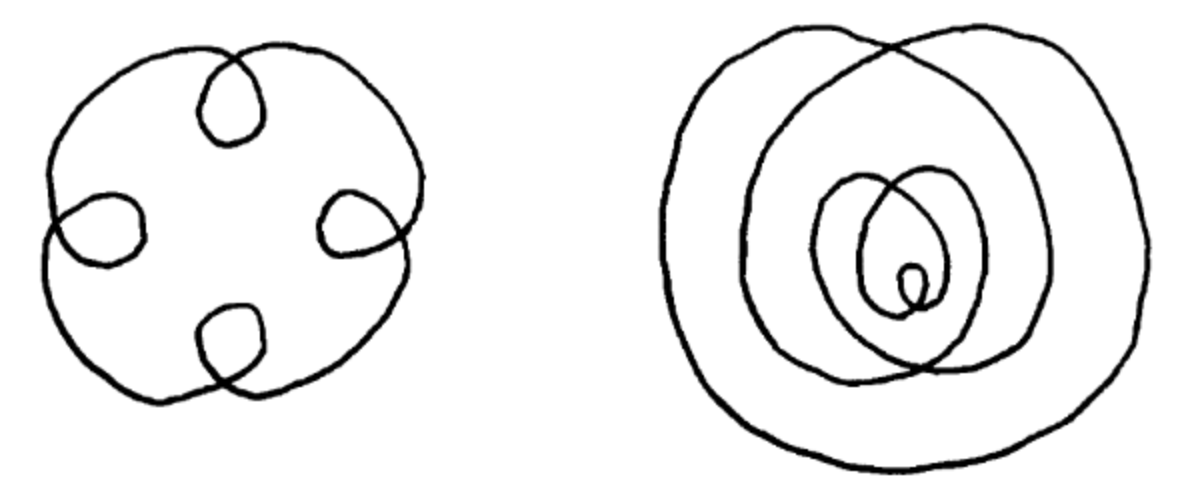
Working towards the goal of characterising which curves admit winning strategies for all starting configurations, it is natural to wonder which characteristics and invariants of a curve might have repercussions on this problem. While the rotation number is a fundamental invariant of plane curves, it is also quite coarse: it merely characterises the connected components in the space of immersions (see [4]). It is thus perhaps not so surprising that two curves sharing that invariant would behave very differently regarding our problem. In fact, the classification of curves based on the rotation number is up to homotopy in the class of closed curves, but not up to diffeomorphisms of the whole plane and therefore ignores all about how the curves are situated in the plane. See Figure 6 for an example of two very different curves with the same rotation number.
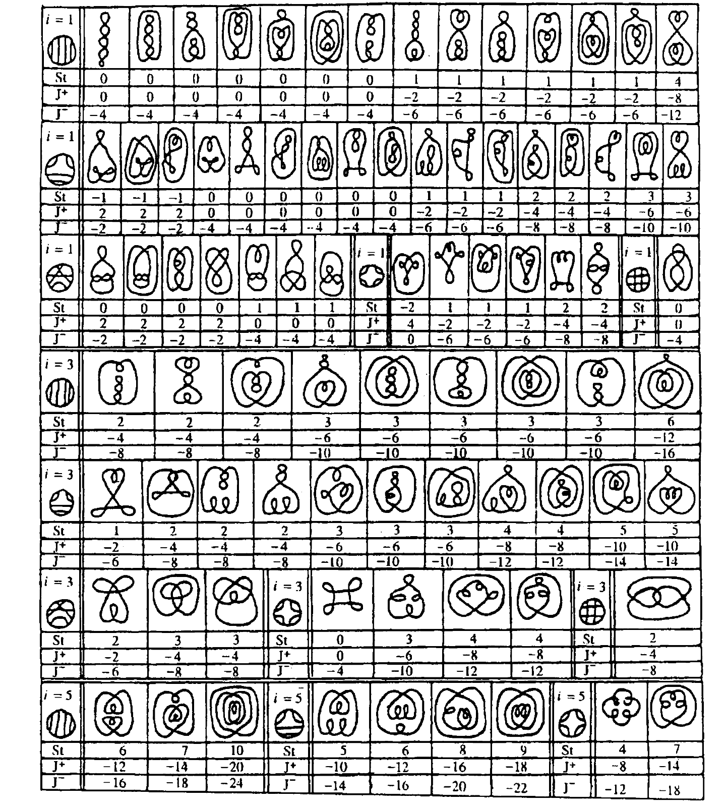
Various finer classifications and invariants have been introduced to address this. Most notably, Arnold’s three invariants classify generic curves in much finer details ([2]; see Figure 7). Together with his use of Gauss diagrams (see [2, p28]), Arnold’s classification for a fixed number of crossings now differentiates many curves previously bundled in the same class and might help provide finer insights into the behaviour of each class of curve with respect to our problem.
Regardless of our preferred choice of curve classification, we can study the behaviour of the problem at hand on the different members of each class.
A priori, there are three possibilities for each class:
-
1.
for every curve in the class, and for every initial configuration on the curve, there exists a strategy to catch the ball; or
-
2.
there is at least one curve in the class such that for every initial configuration there is a strategy to catch the ball, and at least one curve in the class for which there exists a starting position from which we cannot catch the ball; or
-
3.
for every curve in the class, there is a starting position from which we cannot catch the ball.
However, it is easy to see that the third option cannot occur.
Lemma 3.
In every class, there is at least one curve such that for every starting position we can catch the ball.
Take any (geometric) curve in the class. Now find a point on the convex hull, and make a small opening. Attach a huge loop to this opening (radius at least twice the diameter of the original curve).
We claim that on this adapted curve, we can catch the ball by simply keeping walking in one direction. The reason is that, while we are in the original curve, the ball will never go “around” the big loop, since the farthest point on the loop is always too far away. So, we might walk around the big loop once while the ball is somewhere in the original curve, but by the time we enter the big loop for the second time, we must have encountered the ball along the way. ∎
Because of this observation, there are only two possible states for each class: “always yes” or “depends on the geometry”.
To conclude this report, we believe it would be important to understand this classification in more detail; as a small first step towards this goal we present a table with the known behaviours of a few classes of curves (grouped in a coarser 2-parameter table with respect to index and crossing number) in Figure 8.
References
- [1] Mikkel Abrahamsen, Jeff Erickson, Irina Kostitsyna, Maarten Löffler, Tillmann Miltzow, Jérôme Urhausen, Jordi Vermeulen, and Giovanni Viglietta. Chasing Puppies: Mobile Beacon Routing on Closed Curves. Journal of Computational Geometry, vol 13(2):115–150, 2022.
- [2] Vladimir I. Arnold. Plane curves, their invariants, Perestroikas, and classifications. http://www.pdmi.ras.ru/˜arnsem/Arnold/Arnold-PC93.pdf, 1994.
- [3] Damián Wesenberg. A new formula for rotation number. arXiv:2010.01422, 2020.
- [4] Hassler Whitney. On regular closed curves in the plane. Compositio Mathematica, vol 4:276–284, 1937.
4.4 A practical implementation of the link thickening problem
Clément Maria (INRIA – Sophia Antipolis, FR) and Benjamin Burton (The University of Queensland – Brisbane, AU)
License: Creative Commons BY 4.0 International license © Clément Maria and Benjamin Burton
We give a practical solution to the link thickening problem: Given a collection of embedded closed curves in , compute the maximal value such that the -thickening of and have the same homotopy type.
By -thickening, we mean the neighborhood of in , made of all points at distance at most from . We call the supremum of for which the -thickening of and have same homotopy type.
The main goal is to implement an experimentally fast rendering algorithm to visualize knots and links in the Regina [3] library. Our main constraint is that our solution to the link thickening problem should be close to real time in practice.
4.4.1 Persistent homology approach
Persistent homology [4] studies the evolution of the homology of the level-sets
of a continuous function on a topological space . A most studied situation is when the space is the Euclidean space , and the function is the Euclidean distance function to some compact subset of . Available implementations, such as in the Gudhi library [5], essentially work with finite point set approximations of compacts.
In our framework, the ambient space is the 3-dimensional Euclidean space , the compact subset is the collection of closed polygonal curves forming the link, and an -thickening of is the level set of the function assigning to any point the distance from to .
We propose a heuristic solution to the link thickening problem with good practical performance, based on persistent homology. For implementation reasons, it is easier to work with neighborhoods of point clouds, instead of polygonal curves. We start by subsampling the polygonal curves of with a collection of regularly spaced points . Let be the density of in , i.e., the maximal distance between and :
Heuristically, we assume by subsampling sufficiently.
Call the distance function to the point cloud. Let be the cardinality of , and the number of connected components of the link .
In practice, the topology of the level sets , consisting of the union of balls of radius centered at the points in , follows several phases for :
- Phase 1
-
for , the level set is a collection of strictly more than connected components,
- Phase 2
-
for , the level set has the homotopy type of ,
- Phase 3
-
for , the level set does not have the homotopy type of .
Intuitively, the phase consists of disjoint radius -balls centered at the points in when is close to , that eventually merge into a regular neighborhood of the link , once .
For , and under valid density assumptions [1], the level set , or equivalently the union of balls of radius centered at the points of , is guaranteed to have the same homotopy type as the link , i.e.,, a collection of circles.
When passing the critical value , the topology of changes by definition, which happens in three possible ways: generically,
- Case 1
-
either one component of the link fills up, in which case a solid torus neighborhood of turns into a 3-ball,
- Case 2
-
or a component of the link self intersects, in which case a solid torus neighborhood of turns into a genus 2 handlebody,
- Case 3
-
or two distinct components of the link connect to form a genus 2 handlebody.
All three cases are captured by the homology of . Indeed, in case 1, the dimension of the first homology group is reduced by . In case 2, the dimension of increases by . Finally, in case 3, the number of connected components, which is equal to the dimension of the homology group , decreases by .
All cases are readily available from the persistent diagrams of the level sets of the function .
4.4.2 Implementation with Gudhi
The Cech complex based on and of threshold is a simplicial complex which has the same homotopy type as the level set . However, it is challenging and relatively slow to implement its construction, in comparison to the Rips complex [4]. Rips complexes can be interpreted as an approximation of the Cech complex, and are generally preferred in software implementation. When their construction is extremely fast [2], they result into noisier persistence diagrams. However, in our context where is a noiseless subsample of a link in , we do not observe experimentally significant differences in the persistence diagrams of the two filtered complexes.
We interface the Gudhi library with Regina to implement the algorithm above. For efficiency reasons, we stop the computation when the change of homology at is detected. First experiments show a close to real time performance on simple knots and links. See Figure 10 for an example of rendering.

References
- [1] Jean-Daniel Boissonnat, Frédéric Chazal, and Mariette Yvinec. Geometric and Topological Inference. Cambridge Texts in Applied Mathematics. Cambridge University Press, 2018.
- [2] Jean-Daniel Boissonnat and Clément Maria. The simplex tree: An efficient data structure for general simplicial complexes. Algorithmica, 70(3):406–427, 2014.
- [3] Benjamin A. Burton, Ryan Budney, William Pettersson, et al. Regina: Software for low-dimensional topology. http://regina-normal.github.io/, 1999–2023.
- [4] Herbert Edelsbrunner and John Harer. Computational Topology – an Introduction. American Mathematical Society, 2010.
- [5] Clément Maria, Jean-Daniel Boissonnat, Marc Glisse, and Mariette Yvinec. The Gudhi library: Simplicial complexes and persistent homology. In Hoon Hong and Chee Yap, editors, Mathematical Software - ICMS 2014 – 4th International Congress, Seoul, South Korea, August 5-9, 2014. Proceedings, volume 8592 of Lecture Notes in Computer Science, pages 167–174. Springer, 2014.
4.5 Complexity of Reconfiguration Problems
Lena Schlipf (Universität Tübingen, DE), Mikkel Abrahamsen (University of Copenhagen, DK), Kevin Buchin (TU Dortmund, DE), Maike Buchin (Ruhr-Universität Bochum, DE), Linda Kleist (TU Braunschweig, DE), Maarten Löffler (Utrecht University, NL), and André Schulz (FernUniversität in Hagen, DE)
License: Creative Commons BY 4.0 International license © Lena Schlipf, Mikkel Abrahamsen, Kevin Buchin, Maike Buchin, Linda Kleist, Maarten Löffler, and André Schulz
Numerous -hardness proofs for polygons use a reduction from (a version of) planar 3SAT. An instance of planar 3SAT (or a version thereof) is given and a polygon is build on top of , but then the bounded faces of turn (most of the times) into holes in the polygon. Thus, most proofs work only for polygons with holes. However, there are quite some problems that seem to be hard even for simple polygons. But for proving their hardness new ideas are needed. New insights and techniques for such hardness proofs for simple polygons were recently presented by Abrahamsen and Stade [1]. They show that packing unit squares in a simple polygon is -hard by a reduction from monotone planar 3SAT. This working group focuses on how to extend their result to other similar problems.
The first problem that we investigate is motion planning for unit square robots. Given a set of unit squares (robots) in a workspace and a set of target positions, the goal is to move the robots such that (i) each target position is occupied by some robot (unlabeled version), or (ii) each target position is occupied by a specific robot (labeled version). If the workspace is a domain with obstacles, the problem is known to be -hard for both variants, labeled and unlabeled [3, 7]. Building on the result of [1], we could show the following.
Theorem 1.
Motion planning for labeled unit square robots in a simple polygon is -hard.
The proof follows quite easily from the -hardness result of packing unit squares in a simple polygon [1]. The basic idea is to add a small tunnel to the polygon of a packing instance. The robots are then initially placed in the tunnel on the target positions but need to be reordered. The robots can only be reordered if all of them move into the original polygon and then move back into the tunnel in the required reordered manner. Hence, the reordering is only possible if the robots can be packed into the original polygon. ∎
We also investigate -hardness. Many SAT reconfiguration problems are known to be -complete: Given a SAT formula and two satisfying assignments, the question is whether it is possible to find a sequence of flips that takes us from one assignment to the other where a flip allows to change the value of exactly one variable. This is equivalent to the problem of deciding whether the two satisfying assignments are connected in the flip graph of the given SAT formula. We denote this problem by SAT-Reconfiguration; and analogously, we denote the problem for other SAT variants.
The proof for Theorem 1 uses a reduction from monotone planar 3SAT, thus, using the reconfiguration problem of the same version of 3SAT seems like a good choice for proving -hardness of the problem of Theorem 1. It was not known whether the reconfiguration problem of monotone planar 3SAT is -complete, hence, we first show the following result.
Theorem 2.
Deciding whether two satisfying assignments are connected in the flip graph of a monotone planar 3SAT formula is -complete.
The proof is a reduction from Nondeterministic Constrained Logic (NCL) [5, 6]. An NCL instance is given by a directed planar graph and an edge of . The edges are colored blue or red, where every vertex is either incident to three blue edges or to one blue and two red edges. A feasible orientation must respect an indegree of at least two at every vertex, where blue edges count with multiplicity 2. An NCL-instance is positive, if and only if there is a sequence of edge-reversals that finally reverses and any intermediate orientation is feasible.
We first describe a mapping from to a planar 3-SAT formula with embedding by substituting every vertex with incident half edges as shown in Figure 11. For every oriented edge in we introduce one variable in the formula. This variable appears as at the clause nodes induced by and as at the clause nodes induced by . The truth assignment of the formula decodes, which edges are reversed (false variables are the reversed edges). The reversal of an edge in is represented by flipping a variable.
It remains to show that can be turned into a monotone planar 3-SAT formula; for an illustration, consider Figure 12. In a first step, we subdivide the edges in and replace every edge by edges and . We then substitute and as before, but the variable node at is called and the (now distinct) variable node at is now called . The new vertex will be associated with a clause node . In the clauses defined by the original nodes of all variables are nonnegated.
We can now derive a truth assignment from the orientation of as follows: If the edge is not reversed in , we set and . If the edge is reversed in we set and . In order to get an orientation from a satisfying truth assignment we use the same mapping but we could also have and as a satisfying assignment for . In this case the edge would not contribute to the indegree constraint at neither nor in . Thus, we can orient arbitrarily, say in the original orientation.
Our construction yields faces (for the embedding ) of even degree. Hence the dual graph is Eulerian and supports an Euler tour. This tour can be selected such that it can be shortcutted to a cycle that visits all variable nodes without crossing any edge of the embedding of (see Figure 12(b)). ∎
We believe that using Theorem 2 and exploiting the ideas of Abrahamsen and Stade [1] leads to a -hardness proof of the problem of Theorem 1.
In Table 1, we give a summary of some variants of 3SAT and the complexity of their satisfying and reconfiguration problems. Interestingly, most satisfying and reconfiguration problems are hard, but there are some surprising exceptions.
| Satisfying | Reconfiguration | |
|---|---|---|
| 3SAT | -complete | -complete |
| planar 3SAT | -complete | -complete |
| mon. planar not-all-equal 3SAT | -complete | |
| mon. planar 3SAT | -complete | -complete |
| positive 1-in-3SAT | -complete | |
| positive not-all-equal 3SAT | -complete | -complete |
Additionally, we consider the motion planning problem for unit disk robots. Recently, it was proven that the unlabeled motion planning problem for disk robots with two different radii in a domain with obstacles is -hard [2]. We turn our attention to unit disk robots and have some ideas of showing that the problem remains -hard.
Theorem 3.
Reconfiguration of unit disk robots in an arc-gon/polygon with holes is -complete.
We reduce from Constrained Logic. For this we need gadgets to represent two types of vertices (AND and OR gadgets), and edge gadgets that connect them.
Our construction closely follows Brocken et al. [2]; that is, vertices are represented by rooms and edges are represented by tunnels that are filled with disks. The main difference is that we require a gadget that ensures an edge can only have one orientation at a time.
Our new edge gadget is illustrated in Figure 13. Note that the tunnel is shaped (i.e. has small dents) such that the middle three discs cannot move too far out. We claim that:
Claim.
An edge gadget can have all disks “pushed towards the right”, or all disks “pushed towards the left”, or it can have the left half pushed towards the left and the right half pushed towards the right; this is required as an intermediate state when we reconfigure from one state to the other (this corresponds to reorienting the edge in the constraint logic graph). But it is not possible to have all disks in the middle.
The AND and OR gadgets are similar to the ones from Brocken et al. [2]. ∎
References
- [1] Mikkel Abrahamsen and Jack Stade. Hardness of Packing, Covering and Partitioning Simple Polygons with Unit Squares. In preparation.
- [2] Thomas Brocken, G. Wessel van der Heijden, Irina Kostitsyna, Lloyd E. Lo-Wong, and Remco J. A. Surtel. Multi-Robot Motion Planning of k-Colored Discs Is PSPACE-Hard. 10th International Conference on Fun with Algorithms, FUN: 15:1–15:16
- [3] Josh Brunner, Lily Chung, Erik D. Demaine, Dylan H. Hendrickson, Adam Hesterberg, Adam Suhl, and Avi Zeff. 1 X 1 Rush Hour with Fixed Blocks Is PSPACE-Complete. 10th International Conference on Fun with Algorithms, FUN: 7:1–7:14, 2021.
- [4] Parikshit Gopalan, Phokion G. Kolaitis, Elitza Maneva, and Christos H. Papadimitriou. The Connectivity of Boolean Satisfiability: Computational and Structural Dichotomies. SIAM Journal of Computing 38(6):2330–2355 (2009).
- [5] Robert A. Hearn and Erik D. Demaine. The nondeterministic constraint logic model of computation: Reductions and applications. Automata, Languages and Programming, 29th International Colloquium, ICALP 2002: 401–413.
- [6] Robert A. Hearn and Erik D. Demaine. Games, puzzles, and computation. CRC Press, 2009.
- [7] Kiril Solovey and Dan Halperin. On the hardness of unlabeled multi-robot motion planning. Int. J. Robotics Res. 35(14): 1750–1759 (2016).
4.6 Complexity of Testing 0-Efficiency
Eric Sedgwick (DePaul University – Chicago, US), Benjamin Burton (The University of Queensland – Brisbane, AU), Alex He (The University of Queensland – Brisbane, AU), Clément Maria (INRIA – Sophia Antipolis, FR), Tim Ophelders (Utrecht University, NL), Saul Schleimer (University of Warwick – Coventry, GB), Jonathan Spreer (University of Sydney, AU), and Stephan Tillmann (University of Sydney, AU)
License: Creative Commons BY 4.0 International license © Eric Sedgwick, Benjamin Burton, Alex He, Clément Maria, Tim Ophelders, Saul Schleimer, Jonathan Spreer, and Stephan Tillmann
This working group was formed to discuss the complexity of testing the 0-efficiency of a 3-manifold triangulation. This problem appears to be quite challenging, and the group ended up discussing, and making progress on a number of related problems.
Each of these problems concern normal surface theory, a frequently used technique for 3-manifold decision problems. In normal surface theory, a 3-manifold is given via a triangulation, and conclusions about the manifold can be drawn by understanding the normal surfaces, those properly embedded surfaces that intersect each tetrahedron in triangles and/or quadrilaterals.
4.6.1 0-Efficiency, Non-vertex linking normal surfaces
A connected normal surface is vertex linking if it contains only triangles. In a closed 3-manifold, a vertex linking surface will be sphere that is the boundary of a regular neighborhood of some vertex of the triangulation. Each vertex of a triangulation has a vertex linking sphere surrounding it, are there any other normal spheres? A 3-manifold triangulation is 0-efficient if there are none, i.e., all of its normal spheres are vertex linking. Almost all 3-manifolds have a 0-efficient triangulation and working with one yields significant computational advantages [5, 2].
The working group was formed to consider the computational complexity of the following problem:
Problem 1.
Given a 3-manifold triangulation, is it 0-efficient?
Alternatively, we can consider the complementary problem:
Problem 2.
Given a 3-manifold triangulation, does it contain a non-vertex linking 3-sphere?
The work of Hass, Lagarias, and Pippenger [4] shows that if there is a non-vertex linking normal sphere, then there is one with an (exponentially) bounded number of triangles and quadrilaterals. This determines a coordinate vector with linear bit-length which is sufficient to certify that the underlying normal surface is a non-vertex linking sphere. It follows that Problem 2 is in NP (and Problem 1 is in co-NP).
The working group endeavored to show that Problem 2 is also NP-hard, primarily by demonstrating a reduction from a problem such as 3-SAT. One possible model is the work of Agol, Hass and Thurston [1], who used a reduction from 3-SAT to show that the problem 3-Manifold Knot Genus is NP-hard. Unfortunately, it seems quite challenging to adapt their approach to Problem 2. In particular, their reduction yields surfaces with large genus, whereas Problem 2 would require a reduction that always produced a sphere.
The group also considered various analogues and/or variations on Problems 1 and 2, see the sections below. Towards the end of the group’s meetings, a proposal was made to weaken Problem 2 to allow surfaces of higher genus:
Problem 3.
Given a 3-manifold triangulation, does it contain a normal surface that is not subcomplex linking?
A subcomplex linking surface is a normal surface that links a subcomplex of the triangulation. Vertex linking spheres are the simplest case, and always exist, but it is also possible that a normal surface links an edge or even a larger subcomplex of the triangulation.
4.6.2 Composite Knot Recognition
The working group also considered the computational complexity of deciding whether a given knot is composite. In particular, we believe that the following problem is in NP:
Problem 4.
Given a knot , is composite, i.e., can be expressed as a sum of non-trivial knots ?
Typically a knot is specified by providing a knot diagram, a projection of the knot into the plane, with its over and under crossings indicated. A few observations are helpful:
-
1.
A composite knot is characterized by the existence of an decomposing annulus, a meridional essential annulus that is properly embedded in the knot exterior, , where is an open tubular neighborhood of . The knot exterior is a compact manifold with a single torus boundary component. Cutting the exterior along the decomposing annulus, cuts the knot exterior into the exteriors of the knots and .
-
2.
Given a diagram of a knot drawn in the plane with crossings, it is straightforward to produce a triangulation of the knot exterior with at most tetrahedra [4].
Using these observations we can recognize a composite knot by decomposing along this annulus. In particular, we need to
-
1.
Produce the decomposing annulus , and
-
2.
Show that when is cut along , each of the resulting components is a non-trivial knot exterior.
We may assume that the knot exterior is given by a 0-efficient triangulation. Then, some decomposing annulus is realized as a fundamental normal surface. In particular, this means that its coordinates (number of triangles and quadrilaterals) are bounded exponentially and the bit size of the coordinate vector is linear in the number tetrahedra. The coordinate vector of this annulus will serve as the NP certificate. Indeed, using the coordinate vector, we can verify that it represents an incompressible annulus.
It remains to show that when is cut along , the two knot exteriors produced are non-trivial (equivalently, that the annulus is not peripheral in ). For this we can use Lackenby’s result that the unknotting problem is in co-NP [8]. Unfortunately, naively cutting along will not be sufficient as the resulting triangulation is only exponentially bounded. Three alternatives were proposed to mitigate this complication:
-
1.
Cut in a smarter way so that the resulting triangulation (or handle structure) has polynomial (linear?) complexity in terms of the original.
-
2.
Crush along the annulus instead of cutting along it [5, 2]. This is equivalent to Dehn filling the meridian (producing ) and then crushing along a capped off sphere. This reduces the number of tetrahedra, but we would need to prove that knowledge of the summands can be tracked through the crushing procedure.
-
3.
Work with a spun normal annulus in an ideal triangulation. We would need to show that a peripheral annulus would not occur as a spun normal annulus.
Each of these approaches holds promise and would require working out some significant details. Regardless, this result appears to be the most attainable considered by the group.
4.6.3 Ribbon Knot Recognition
The working group also discussed the complexity of ribbon knot recognition with the aim of showing that this problem is in NP for small knots:
Problem 5.
Given a small knot , is a ribbon knot?
A small knot is a knot with no closed essential surfaces in its exterior. Every knot bounds an immersed disk. A knot is a ribbon knot, if it bounds a ribbon disk an immersed disk with only ribbon singularities. A ribbon singularity is an arc of self intersection whose pre-image in the disk consist of two arcs, one arc in the interior of the disk (a slit) and one arc with both endpoints in the boundary of the disk (the ribbon passing through the slit).
Given a ribbon knot, choose a ribbon disk that minimizes the number of ribbon singularities. Each of the, say , ribbon singularities can be desingularized, in two distinct ways, by a cut and paste of the two sheets that meet the singularity. Resolving all singularities produces a Seifert surface for the knot with Euler characteristic .
Question 6.
Among the choices for desingularization, is there always one that produces an incompressible surface?
While there are clear cases where bad choices produce a compressible surface, an affirmative answer yields an approach to ribbon knot recognition.
Suppose that there is a desingularization producing an incompressible surface . When the knot is small, will be realized by a fundamental normal surface. (If is a normal sum, then one of the summands is a closed essential surface contradicting that is small [7, 6]).
The goal would then be to exhibit an NP certificate consisting of the fundamental normal surface along with a collection of disks in its complement that demonstrate how to resingularize the surface to produce a ribbon disk for .
References
- [1] Ian Agol, Joel Hass, and William Thurston. 3-manifold knot genus is NP-complete. In Proceedings of the Thirty-Fourth Annual ACM Symposium on Theory of Computing, pages 761–766. ACM, New York, 2002.
- [2] Benjamin Burton. A new approach to crushing 3-manifold triangulations. Discrete Comput. Geom., 51(4):864–892, 2014.
- [3] Benjamin A. Burton. Introducing Regina, The 3-Manifold Topology Software. Experimental Mathematics, 13(3):267 – 272, 2004.
- [4] Joel Hass, Jeffrey C. Lagarias, and Nicholas Pippenger. The computational complexity of knot and link problems. Journal of the ACM (JACM), 46(2):185–211, 1999.
- [5] William Jaco and J. Hyam Rubinstein. -efficient triangulations of 3-manifolds. J. Differential Geom., 65(1):61–168, 2003.
- [6] William Jaco and Eric Sedgwick. Decision problems in the space of Dehn fillings. Topology, 42(4):845–906, 2003.
- [7] William Jaco and Jeffrey L. Tollefson. Algorithms for the complete decomposition of a closed -manifold. Illinois Journal of Mathematics, 39(3):358 – 406, 1995.
- [8] Marc Lackenby. The efficient certification of knottedness and Thurston norm. Advances in Mathematics, 387:107796, 2021.
4.7 Two problems on flip distances
Jonathan Spreer (University of Sydney, AU), Jean Cardinal (ULB – Brussels, BE), Francis Lazarus (CNRS – Grenoble, FR), Lionel Pournin (Université Paris 13 – Villetaneuse, FR), Günter Rote (FU Berlin, DE), Saul Schleimer (University of Warwick – Coventry, GB), and Birgit Vogtenhuber (TU Graz, AT)
License: Creative Commons BY 4.0 International license © Jonathan Spreer, Jean Cardinal, Francis Lazarus, Lionel Pournin, Günter Rote, Saul Schleimer, and Birgit Vogtenhuber
These are the notes of the working group looking into flip distances. They contain two initial findings. The first one is a family of pairs of triangulations of the convex -gon, where is at least , that produces flip paths of worst possible length between them for a natural heuristic. The second one consists of upper and lower bounds on the flip distances in the modular flip graph of the annulus with arbitrary numbers of marked points on its boundary components.
4.7.1 Introduction
Flip graphs – graphs whose vertices are the triangulations of a geometric or topological space and whose edges correspond to a local operation between them called a flip – appear naturally in computational geometry [15, 20, 24] and in low-dimensional topology [2, 9, 17]. When the triangulated space is a convex polygon, that graph is also relevant to algebraic combinatorics since in that case, it is precisely the edge graph of the associahedron [14], a polytope that has been generalized in a number of ways [5, 10, 11, 21].
The geometry of flip graphs has attracted considerable attention because it is intimately connected to the complexity of balancing binary trees [27], provides a dissimilarity measure between these trees [7], serves as a combinatorial model for the mapping class group of a surface [9, 17], or can be used as a tool to optimize triangulations [1, 3, 4]. The diameter of the associahedron is known exactly [23], but the complexity of computing the distance between two of its vertices is still an open problem [15, 20].
This note has two parts. In Section 4.7.2, we discuss two natural heuristics to find short paths between triangulations of the convex -gon and show how they are linked. The heuristics use what is called shadow vertex paths and crossing-monotone flip sequences. We then present a family of pairs of triangulations for which one of these heuristics performs worst possible, up to a constant factor, and discuss implications for the other heuristics. In Section 4.7.3 we prove upper and lower bounds on flip distances in the modular flip graph of triangulations of the annulus with and marked points on its boundary components, . More specifically, we prove that the diameter of this flip graph must lie between and , see Lemmas 9 and 10.
4.7.2 Negative results for flip path heuristics
In this section, we consider the flip graph of a Euclidean convex -gon . A triangulation of is a set of pairwise non-crossing arcs between the vertices of that decompose into triangles. In this context, an arc is just a straight line segment. The vertices of are the triangulations of and its edges link and pair of triangulations that differ by exactly one arc. It is well-known that is the edge graph of the -dimensional associahedron [14].
We consider two natural heuristics for computing short flip sequences between two given triangulations and of a convex -gon:
-
1.
Shadow vertex paths are obtained by projecting the associahedron onto a plane. The two directions defining the projection (the shadow) are chosen such that vertices corresponding to and are both extremal. Then, the projection is used to describe a sequence of flips turning into . The resulting flip path depends on the chosen realization of the associahedron and on the choice of directions for and in their respective normal cones. A natural choice of realization of the associahedron is the realization as a secondary polytope for a regular -gon.
-
2.
Superimpose and . A crossing-monotone path is a sequence of flips, strictly reducing the number of crossing pairs of arcs between and the intermediate triangulations obtained from at each step.
We show how these two heuristics are linked, obtain negative results for the first heuristic, and discuss the implications on the second. More precisely, we present pairs of triangulations, where the path constructed by the first heuristic is of length . This path realizes the worst case asymptotics and is much longer than the actual shortest path of length .
4.7.2.1 Crossing-monotone paths
It is known that crossing-monotone paths exist for all pairs of triangulations of a set of points in [12]. The same holds for topological surfaces [2, 9, 16]. In this section we give a short proof of this fact in the special case of a convex -gon. Given are two triangulations and of the convex -gon. We start with and flip edges until we reach the target triangulation . We refer to and all intermediate triangulations as the red triangulation and to as the blue triangulation.
We start by superimposing and . We enumerate the set of red edges with the maximum number of blue intersections. Each of these edges splits the -gon into two pieces. We call such an edge outermost, if one of the two pieces does not contain any red edge with maximum number of intersections.
Lemma 1.
Flipping an outermost red edge decreases the number of intersections between the red and blue triangulations by at least one.
Let be an outermost red edge with maximum number of blue intersections, and let and be its endpoints. Let and be the two red triangles containing with vertices , , , and , , respectively. Without loss of generality, let be the vertex on the outermost side. Denote the number of blue edge segments separating one of the four corners , , , and of the quadrilateral from the other three by , , , and , respectively. The quadrilateral may also have transversing edge segments in one of two directions. Without loss of generality, let these intersect the edges running between and , and and , respectively. See Figure 15 for an illustration.
We then have for the number of intersections of the edges of and : is intersected times. The edge between and is intersected times (note that outermost edges must have strictly fewer than intersections by construction). It follows that we have . Similarly, the edge between and is intersected times and hence . It follows that flipping creates an edge which is intersected times and the overall number of intersections between the red and blue triangulations has strictly decreased. ∎
From Lemma 1 the existence of crossing-monotone paths immediately follows: iteratively flip an outermost red edge with maximum number of crossings, until the red and blue triangulations coincide. Since and initially have crossings, this is also an upper bound for the length of such a path.
4.7.2.2 Shadow vertex paths
Secondary polytopes and regular triangulations.
Regular triangulations of point sets in are projections of the lower convex hulls of lifted point sets, in which every point is assigned an arbitrary height as th coordinate. It is well-known that regular triangulations are one-to-one with vertices of the secondary polytope [11]. The latter is realized as the convex hull of points whose coordinates are the combined volume of the simplices incident to each point in the triangulation. The edges of the secondary polytopes are one-to-one with bistellar flips. Note that, in the general case, flips are no longer always edge flips and a more general definition is needed for them (see for instance [24, Definition 4]). In particular, flips can remove or introduce a vertex in a triangulation, provided that this vertex is not a vertex of the convex hull of the considered set of points. For a comprehensive introduction to flips and flip graphs in arbitrary dimensions, see [8].
The method.
A shadow vertex paths on the secondary polytope is obtained by linearly interpolating between height functions of the two triangulations corresponding to the two endpoints. A height function can be interpreted as a direction in space, such that the lower convex hull defines the triangulation associated with the optimal vertex of the secondary polytope in this direction. Recall that a path in the edge graph of a polytope is non-revisiting when the vertices of that path that belong to any given facet of are consecutive. In other words, such a path never re-enters a facet of after it leaves it.
Lemma 2.
Shadow vertex paths on the secondary polytope of a set of points in general position are non-revisiting. This implies that a shadow vertex path on the secondary polytope of a set of points in convex position in the plane always has length at most .
This follows from the known fact that, when a face of a triangulation disappears along a shadow vertex path, this face cannot reappear later in that path [24, Theorem 8]. Facets of secondary polytopes are one-to-one with subdivisions that can only be coarsened by the trivial subdivision [8]. Consider such a subdivision that corresponds to a facet of the secondary polytope. When the point set that gives rise to the secondary polytope is in general position, a face of that is not full-dimensional must be a simplex. The shadow vertex path leaves precisely when one of these simplices disappears. As they cannot reappear later along the path, cannot be revisited.
For the secondary polytope of points in convex position in the plane, the facets correspond to the diagonals of the polygon. Since a vertex of is incident to facets and the shadow vertex paths on are non-revisiting, such a path has length at most
as desired. ∎
Implications and scope of the method.
We recall that a polytope is Hirsch when the diameter of its edge graph is at most the number of its facets minus its dimension [13, 26].
Theorem 3.
Secondary polytopes of point sets in general position are Hirsch.
The existence of a non-revisiting path between every pair of vertices implies Hirsch’s bound on the diameter [13, 26]. ∎
Recall that a polytope is non-revisiting if all the geodesics paths between its vertices are non-revisiting (this is called the non-leaving face property in [6]).
Lemma 4.
There exist secondary polytopes of -dimensional point sets, for some , that are not non-revisiting.
This is obtained with the so-called mother of all examples [8]: point sets consisting of two homothetic simplices one of whose is contained in the interior of the other. Their secondary polytope is known as the stellohedron [22], and is known to have revisiting geodesics [6]. ∎
This shows that for higher-dimensional regular triangulations, there exist geodesics that are not shadow vertex paths.
Lemma 5.
There exist secondary polytopes and geodesics on those, that are not shadow vertex paths. Hence there does not exist any height function whose interpolation yields a shortest flip sequence.
4.7.2.3 A family of examples producing long paths
In this section we present a family of pairs of triangulations of the -gon for which the methods described in Sections 4.7.2.1 and 4.7.2.2 produce paths of asymptotically worst possible length .
Figure 16 shows four members of our family of examples, each consisting of a start and a target triangulation. They consist of triangulations of a -gon, obtained by gluing fan-triangulations of two -gons in a point-symmetric way. Start and end triangulations are identical, except for a rotation of one th of a full twist.

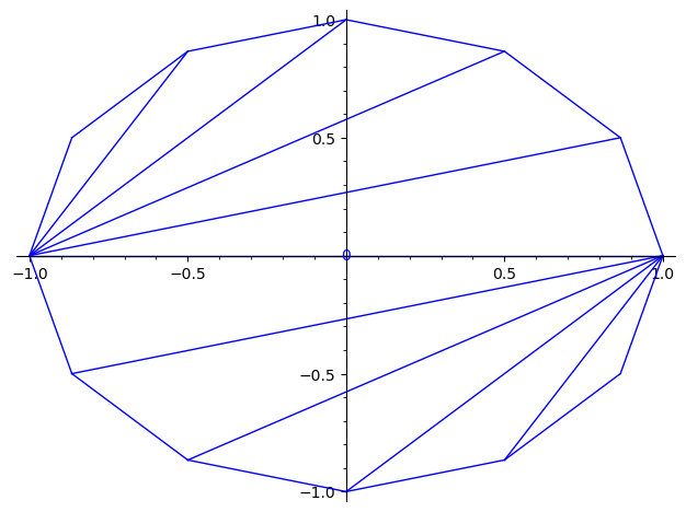
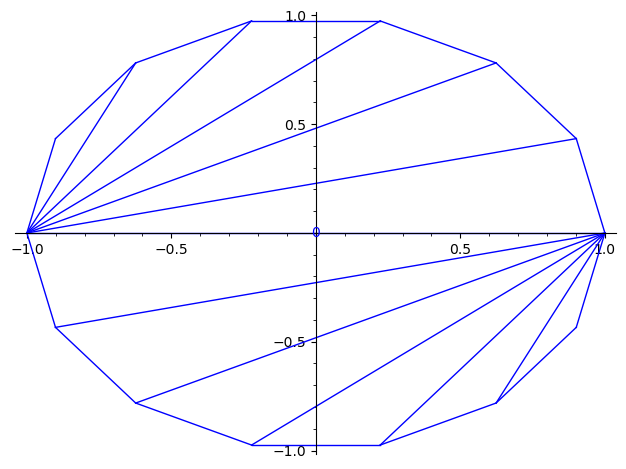
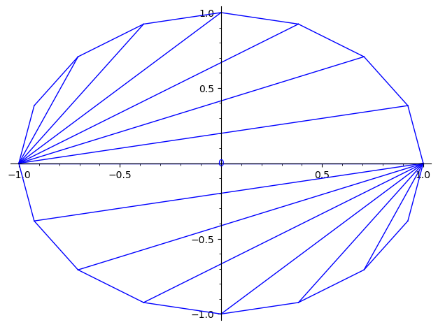
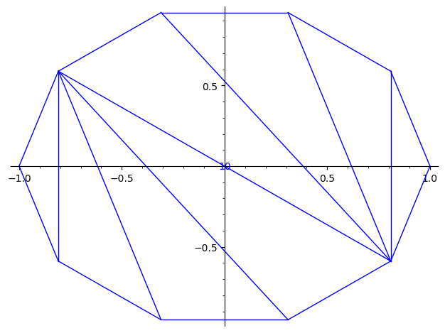
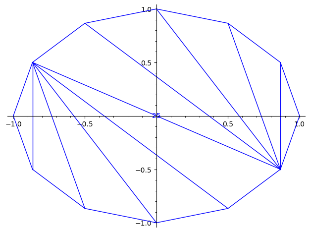
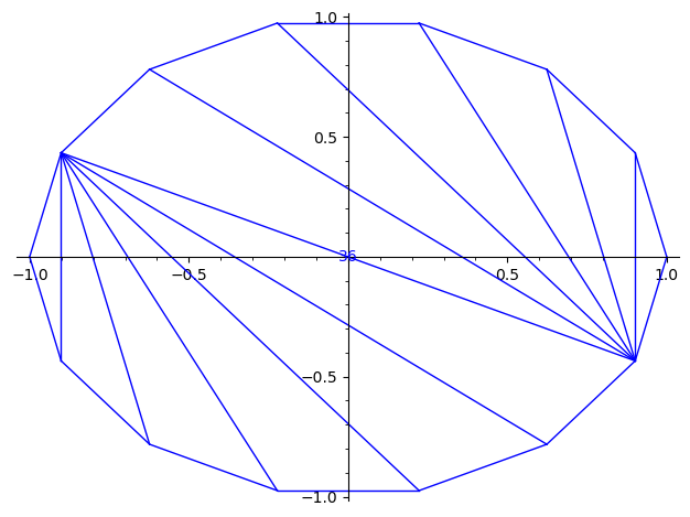
Lemma 6.
There exist shadow vertex paths transforming triangulations of the -gon into in steps.
In particular, there exist shadow vertex paths of length on the (secondary polytope realization of the) associahedron, hence the upper bound from Lemma 2 is tight, up to a factor of .
It is enough to provide a pair of height functions for every pair of triangulations with the desired properties.
We pick vertices of the -gon with coordinates , , and label them from to accordingly. For , vertices and start with heights and end with heights , linearly interpolating between these to values to flip from to . The heights can be perturbed by small amounts to ensure general position throughout the procedure.
We claim without proof that the shadow vertex paths obtained in this way have the desired property. ∎
Remark.
Gradually adding small, random perturbations to the height functions proposed in the proof of Lemma 6 allows us to find other flip sequences using the shadow vertex path method. For instance, a guided search based on iteratively performing small random permutations, finds flip sequences between and of length (a geodesic) and .
Lemma 7.
There exist crossing-monotone sequences of flips between triangulations of a convex -gon that are of quadratic size (and hence worst possible).
The flip sequence from the proof of Lemma 6 is crossing-monotone. ∎
The crossings based heuristics described at the beginning of the section is implemented in practice by selecting at each step a flip that makes the number of crossings decrease the most. In that case, it is known that the heuristics is, at best a -approximation algorithm [25]. However, computational evidence suggests that it is accurate most of the time [7]. This implementation works very well on the examples that we describe here and we ask the following.
Question 8.
Is the greedy crossing heuristic, in which we flip an arc that decreases the number of crossings the most, an approximation algorithm?
4.7.3 The modular flip graph of the annulus
Consider an orientable surface equipped with a finite set of points such that each boundary component of contains at least one of these points. By a triangulation of , we mean an inclusion-wise maximal set of pairwise non-crossing arcs on between two of these prescribed points. Note that the arcs are considered up to isotopy, so in particular, when we say that two arcs are non-crossing, this means that two representatives in the corresponding isotopy classes are non-crossing. The flip graph of is the graph whose vertices are the triangulations of and whose edges correspond to flipping arcs.
The modular flip graph of is obtained by quotienting by the homeomorphisms of that fix the vertices of the triangulations pointwise [17]. It is known that when is an annulus with points on one boundary and a single point on the other, the diameter of the modular flip graph of is exactly [17, Theorem 1.4]. In this section, we consider the slightly more general case when is an annulus with points on one boundary and on the other, with . We aim at bounding the worst-case diameter of the modular flip graph of as a function of .
4.7.3.1 Upper bounds
In this section we prove the following statement.
Lemma 9.
Let be an annulus with a total of marked points on its two boundary. The diameter of is .
Let and be two arbitrary triangulations of the annulus . Let be a vertex on the inner boundary of such that in , is adjacent to at least one vertex on the outer boundary of . (Note that each triangulation of has at least one such vertex ). Let and , and , be the number of vertices on the outer and on the inner boundary component of , respectively.
We start by flipping to a common target. For this we iteratively increase the vertex degree of in until it is adjacent to all other vertices. Note that, as long as is not yet adjacent to all other vertices, it is always possible to find a flip that strictly increases the degree of : every edge that is not a boundary edge is flippable, and the vertex link of contains a non-boundary edge if and only if is not yet adjacent to all other vertices. Since there are non-boundary edges, and may initially not be adjacent to a single one, this can always be done in at most flips.
The result is a triangulation with – necessarily – the following properties:
-
there exists a unique vertex on the other boundary with two edges running between and , enclosing this inner boundary and forming a heart shape
-
every other vertex on the outer boundary has exactly one edge running between it and
-
there is a loop edge running from to and encircling the inner boundary
-
there exists a unique vertex on the inner boundary with two edges running between and
-
every other vertex on the inner boundary has exactly one edge running between it and
Note that the vertices , , and in the above properties uniquely determine . See Figure 17 for an illustration.
For , we cut along the edge to obtain a “rectangle” (cycle with vertices), whose corners are two copies of each of and . Two opposite sides of the rectangle contain the outer and inner boundary points of , respectively, and the other two sides are the two copies of the edge .
Note that the edges of form a triangulation of this rectangle and that flips between triangulations in the rectangle correspond to flips between triangulations of the annulus . Using at most flips, we can flip in this rectangle from to a fan at any of the two copies of . Gluing the resulting triangulation along edge yields a triangulation of where has maximum degree,
Note that we can arbitrarily choose, which copy of we use as the center of the fan. We make this choice in the following way: Consider the number of vertices of that lie between one copy and along the inner boundary part of the rectangle, and the number of vertices of that lie between the other copy of and along the inner boundary part of the rectangle. For the centre of the fan, we choose the copy of for which this number is greater. Note that since , we have .
We can now flip to in the following way: Along the outer boundary of , we keep on flipping one of the two edges between and (initially) until there are two edges running between and . Since we can choose the direction around the outer circle in which we travel, this can be done in at most flips. Next we turn to the inner boundary of : here, similarly as before, we can flip to be twice adjacent to in at most flips. This is possible because of how we chose the centre of the fan. After these additional at most flips, the triangulations now coincide.
Altogether, the flip sequence described above is of length . ∎
4.7.3.2 Lower bounds
The tools to prove lower bounds on the diameter of flip-graphs of surfaces can be found in [17, 18, 19, 23].
The best introduction to the lower bound techniques would be to read [17] first, though the case of the annulus with points on a boundary and one point on the other (matching lower and upper bounds for the diameter of the flip-graph) is treated in [17]. Note also that a general upper bound of 4n+K (K is a constant) on the diameter of the flip-graph is given in [17] in the case when there’s a boundary containing n points and the rest of the surface is arbitrary but fixed. These techniques were introduced in [23] in the special case of convex polygons.
Lemma 10.
There exist triangulations and of the annulus with points on their boundaries that are flips apart.
Start with the diameter realising pair of triangulations of the case , . This requires a flip sequence of length at least [17].
Next we think of the inner boundary to have more than one point. Since there is a loop edge encircling the inner boundary (see [17] for details), the space bounded by the inner boundary together with the loop edge is an -gon of diameter . Since, according to [27], a geodesic between triangulations having a common edge, preserves this edge, the loop edge of these examples remains intact in a shortest path from one to the other. It follows that these triangulations require at least flips to be connected. Since inner and outer boundary are symmetric, this bound is lowest for and hence we obtain a lower bound of . ∎
References
- [1] Eduardo Altmann and Jonathan Spreer. Sampling triangulations of manifolds using Monte Carlo methods. https://arxiv.org/abs/2310.07372, 2023. 29 pages, 6 figures.
- [2] Mark C. Bell. Simplifying triangulations. Discrete & Computational Geometry, 66(1):1–11, 2021.
- [3] Anders Björner and Frank H. Lutz. Simplicial manifolds, bistellar flips and a 16-vertex triangulation of the Poincaré homology 3-sphere. Experiment. Math., 9(2):275–289, 2000.
- [4] Benjamin A. Burton. The Pachner graph and the simplification of 3-sphere triangulations. In SoCG ’11: Proceedings of the twenty-seventh annual symposium on Computational geometry, pages 153–162. ACM, 2011.
- [5] Michael P. Carr and Satyan L. Devadoss. Coxeter complexes and graph-associahedra. Topology and its Applications, 153:2155–2168, 2006.
- [6] Cesar Ceballos and Vincent Pilaud. The diameter of type associahedra and the non-leaving-face property. European Journal of Combinatorics, 51:109–124, 2016.
- [7] Sean Cleary and Roland Maio. Edge conflicts do not determine geodesics in the associahedron. SIAM Journal on Discrete Mathematics, 32(2):1003–1015, 2018.
- [8] Jesús A. de Loera, Jörg Rambau, and Francisco Santos. Triangulations: structures for algorithms and applications, volume 25 of Algorithms and Computation in Mathematics. Springer, 2010.
- [9] Valentina Disarlo and Hugo Parlier. The geometry of flip graphs and mapping class groups. Transactions of the American Mathematical Society, 372(6):3809–3844, 2019.
- [10] Sergey Fomin and Andrei Zelevinsky. -systems and generalized associahedra. Annals of Mathematics, 158:977–1018, 2003.
- [11] Israel M. Gel’fand, Andrei V. Zelevinsky, and Mikhail M. Kapranov. Newton polytopes of principal A-determinants. Soviet Mathematics. Doklady, 40:278–281, 1990.
- [12] Sabine Hanke, Thomas Ottmann, and Sven Schuierer. The edge-flipping distance of triangulations. Journal of Universal Computer Science, 2(8):570–579, 1997.
- [13] Victor Klee and David W. Walkup. The -step conjecture for polyhedra of dimension . Acta Mathematica, 117:53–78, 1967.
- [14] Carl W. Lee. The associahedron and triangulations of the -gon. European Journal of Combinatorics, 10(6):551–560, 1989.
- [15] Anna Lubiw and Vinayak Pathak. Flip distance between two triangulations of a point set is NP-complete. Computational Geometry, 49:17–23, 2015.
- [16] Lee Mosher. Mapping class groups are automatic. Annals of Mathematics, 142(2):303–384, 1995.
- [17] Hugo Parlier and Lionel Pournin. Flip-graph moduli spaces of filling surfaces. Journal of the European Mathematical Society, 19(9):2697–2737, 2017.
- [18] Hugo Parlier and Lionel Pournin. Modular flip-graphs of one holed surfaces. European Journal of Combinatorics, 67:158–173, 2018.
- [19] Hugo Parlier and Lionel Pournin. Once punctured disks, non-convex polygons, and pointihedra. Annals of Combinatorics, 22:619–640, 2018.
- [20] Alexander Pilz. Flip distance between triangulations of a planar point set is APX-hard. Computational Geometry, 47:589–604, 2014.
- [21] Alexander Postnikov. Permutohedra, associahedra, and beyond. International Mathematics Research Notices, 2009(6):1026–1106, 2009.
- [22] Alexander Postnikov, Victor Reiner, and Lauren Williams. Faces of generalized permutohedra. Documenta Mathematica, 13:207–273, 2008.
- [23] Lionel Pournin. The diameter of associahedra. Advances in Mathematics, 259:13–42, 2014.
- [24] Lionel Pournin and Thomas M. Liebling. Constrained paths in the flip-graph of regular triangulations. Computational Geometry, 37(2):134–140, 2007.
- [25] Lionel Pournin and Zili Wang. Strong convexity in flip-graphs. arXiv:2106.08012, 2021.
- [26] Francisco Santos. A counterexample to the Hirsch conjecture. Annals of Mathematics, 176:383–412, 2012.
- [27] Daniel Sleator, Robert Tarjan, and William Thurston. Rotation distance, triangulations, and hyperbolic geometry. Journal of the American Mathematical Society, 1:647–681, 1988.
5 Participants
-
Mikkel Abrahamsen – University of Copenhagen, DK
-
Therese Biedl – University of Waterloo, CA
-
Florestan Brunck – IST Austria – HKlosterneuburg, AT
-
Kevin Buchin – TU Dortmund, DE
-
Maike Buchin – Ruhr-Universität Bochum, DE
-
Benjamin Burton – The University of Queensland – Brisbane, AU
-
Jean Cardinal – ULB – Brussels, BE
-
Hsien-Chih Chang – Dartmouth College – Hanover, US
-
éric Colin de Verdière – Gustave Eiffel University – Marne-la-Vallée, FR
-
Arnaud de Mesmay – CNRS, Gustave Eiffel University – Marne-la-Vallée, FR
-
Fabrizio Frati – University of Rome III, IT
-
Alex He – The University of Queensland – Brisbane, AU
-
Linda Kleist – TU Braunschweig, DE
-
Francis Lazarus – CNRS – Grenoble, FR
-
Maarten Löffler – Utrecht University, NL
-
Anna Lubiw – University of Waterloo, CA
-
Clément Maria – INRIA – Sophia Antipolis, FR
-
Tim Ophelders – Utrecht University, NL
-
Lionel Pournin – Université Paris 13 – Villetaneuse, FR
-
Günter Rote – FU Berlin, DE
-
Saul Schleimer – University of Warwick – Coventry, GB
-
Lena Schlipf – Universität Tübingen, DE
-
André Schulz – FernUniversität in Hagen, DE
-
Eric Sedgwick – DePaul University – Chicago, US
-
Rodrigo I. Silveira – UPC Barcelona Tech, ES
-
Jonathan Spreer – University of Sydney, AU
-
Stephan Tillmann – University of Sydney, AU
-
Birgit Vogtenhuber – TU Graz, AT
-
Zili Wang – Sun Yat-Sen University – Shenzen, CN
-
Erin Moriarty Wolf Chambers – St. Louis University, US
-
Alexander Wolff – Universität Würzburg, DE
![[Uncaptioned image]](x3.jpg)