GDBMiner: Mining Precise Input Grammars on (Almost) Any System

Abstract
If one knows the input language of the system to be tested, one can generate inputs in a very efficient manner. Grammar-based fuzzers, for instance, produce inputs that are syntactically valid by construction. They are thus much more likely to be accepted by the program under test and to reach code beyond the input parser.
Grammar-based fuzzers, however, need a grammar in the first place. Grammar miners are set to extract such grammars from programs. However, current grammar mining tools place huge demands on the source code they are applied on, or are too imprecise, both preventing adoption in industrial practice.
We present GDBMiner, a tool to mine input grammars for binaries and executables in any (compiled) programming language, on any operating system, using any processor architecture, even without source code. GDBMiner leverages the GNU debugger (GDB) to step through the program and determine which code locations access which input bytes, generalizing bytes accessed by the same location into grammar elements.
GDBMiner is slow, but versatile – and precise: In our evaluation, GDBMiner produces grammars as precise as the (more demanding) Cmimid tool, while producing more precise grammars than the (less demanding) Arvada black-box approach. GDBMiner can be applied on any recursive descent parser that can be debugged via GDB and is available as open source.
Keywords and phrases:
program analysis, testing, input grammar, fuzzing, grammar miningFunding:
Max Eisele: Max Eisele conducted this research as part of his PhD thesis at Saarland University.Copyright and License:
2012 ACM Subject Classification:
Software and its engineering Syntax ; Software and its engineering Operational analysis ; Software and its engineering Software testing and debugging ; Computer systems organization Embedded softwareSupplementary Material:
Software (Source Code and Experiment Data): https://github.com/boschresearch/gdbminerarchived at
Funding:
This work was funded by the German Federal Ministry of Education and Research (BMBF, project CPSec - 16KIS1565 and 16KIS1564K).DOI:
10.4230/LITES.10.1.1Received:
2024-05-28Accepted:
2025-01-10Published:
2025-04-16Part Of:
TGDK, Volume 10, Issue 1Journal and Publisher:
1 Introduction
In industry, proper software testing is the number one technique to satisfy safety, security, and privacy requirements. As manual testing is laborious and code constantly grows [42], there is a huge demand for automated software testing solutions.
Having the input specification of a program under test can help to automate testing. A context-free grammar, for instance, can be used to produce large amounts of valid and diverse test inputs [20]. However, formal input specifications are rarely available in practice; and writing grammars by hand is cumbersome.
Recent research has demonstrated that input grammars can be mined from inputs and programs:
-
Autogram [23] traces data flow of different parts of the input into functions and variables and compiles resulting rules to a context-free grammar. However, it is implemented for Java programs only, and therefore, unsuited for a variety of systems and programs.
-
Mimid [18] leverages control flow, as well as data flow instrumentation of the target program to reconstruct derivation trees, and subsequently uses a number of active learning steps – basically testing for interchangeability of subtrees – to translate these into a grammar. Mimid requires the program code to be written in Python or C (Cmimid). However, to be used with Cmimid, the C code cannot have gotos, macros, or enumerations; case statements without braces or with fall-throughs are not allowed. While such restrictions pose little problems for the proof-of-concept of a prototype, they make Cmimid impractical for industrial use.
-
Arvada [28] and TreeVada [5] are black-box approaches that only require oracle requests (tests whether an input is accepted by the target program) to approximate a grammar. They therefore offer an approach to grammar mining that only requires the ability to execute a program. However, by construction, Arvada, and TreeVada have less information available than code-based approaches, and the resulting grammars may thus be less precise.
To mine input grammars in our context, we present a novel approach that does not suffer from the above limitations – and actually is set to be applicable for binaries and executables in any programming language, on any operating system, using any processor architecture, even without source code. The realm of embedded systems is not well definable, but it is clear that they are computerized systems build for specific purposes [48]. Compared to traditional computing systems, the hardware of embedded systems is generally speaking more constrained and diverse. However, the program execution on embedded systems is often controllable via debuggers, which is why the key ingredient of our approach is to use the GNU debugger (GDB) [46] as interface to the program under test, allowing a grammar miner to:
-
1.
Step through the program, identifying the code executed.
-
2.
Use watchpoints to track data accesses during execution.
These features give a grammar miner the ability to associate input data with code locations that process them. This, in turn, allows a grammar miner to group input bytes that are processed by the same code into equivalence classes and hence grammar elements. Also taking the call stacks of the processing code into account, we can produce precise and human-readable input grammars.
Using GDB to step through executions is time-consuming – but once a grammar is mined from a system, it can be used again and again for high-speed generation of valid inputs, offsetting any effort spent to mine the grammar in the first place. The main advantage of using GDB, however, is that it is versatile, providing a unified interface for most software and systems. GDB works with Assembly, C, and C++, popular languages for programming embedded systems, as well as Ada, Objective-C, Rust, Pascal, Modula-2, FORTRAN, Go, and many other compiled programming languages; it can also be applied on binaries without source code. It supports most microprocessor instruction sets, including ARM, x86, Motorola 68000, MIPS, PA-RISC, PowerPC, and RISC-V.
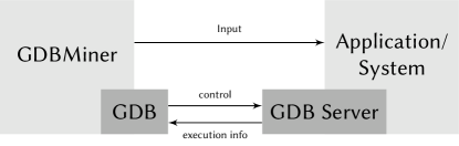
Furthermore, GDB supports remote debugging, where GDB runs on one machine, and the program under test runs on another. GDB then communicates via TCP with a remote GDB Server running on a debug probe or the host computer, e.g. to control the debug unit on a microcontroller that is part of an embedded system (Figure 1).
We have implemented the above grammar mining approach in an open source tool named GDBMiner, bringing input grammar mining to any recursive descent parser that can be debugged with GDB – from C-compiled executables on general-purpose PCs to read-only binaries on embedded systems.
With GDBMiner, we contribute a unified, language- and architecture-agnostic approach for mining input grammars on any system with debugging capabilities. As we show in our evaluation, GDBMiner produces input grammars that are precise, well-structured, and very suitable for test generation, especially for black-box testing. The versatility of GDBMiner and the universality of the resulting grammars enables efficient software testing under adverse conditions, including embedded systems, and thus, specifically addresses the needs of software engineering in practice.
The remainder of this paper is organized as follows. Section 2 summarizes known concepts and techniques, followed by our approach in Section 3. We cover implementation details in Section 4. Section 5 evaluates GDBMiner against the state of the art and contains a walkthrough of a demo application. Section 6 discusses limitations of our approach and Section 7 closes with conclusion and future work.
2 Background
The following background knowledge is essential for this paper.
2.1 Context-free Grammars
Context-free grammars are mathematical descriptions for context-free languages. They can serve for generating inputs that belong to the corresponding language or for verifying if an input belongs to that language. For instance, the language of correctly parenthesized expressions is a popular example of a context-free language. In contrast to regular languages, context-free languages can take care of these matching parentheses, which makes them ideal for describing mathematical expressions, but also the syntax of programming languages. Generating strings from a context-free grammar is easy, and deciding whether a string is producible by a given context-free grammar is efficient [11]. Limits of context-free languages are context-sensitive properties, for instance, arbitrary matching tags as they are used in the XML format, or checksums over the content.
Formally, a context-free grammar is a four-tuple , with variable (or non-terminal) symbols , terminal symbols , the set of productions , and the start symbol [22]. A production rule is a relation with variable mapped to a string of variables and terminals .
As an example, consider this grammar for correctly parenthesized expressions: S ::= SS | S | . Applying on the string ‘(()())’ yields the parse tree in Figure 2.
2.2 Recursive Descent Parsers
Recursive descent parsers are a popular way to implement parsers for context-free grammars in practice [31]. They operate in a top-down manner, recursively calling parser subroutines that match non-terminals, and can precisely parse grammars [26] whose production rules are unambiguous when reading a string one by one. Having a context-free grammar, it is possible to generate sound recursive descent parsers automatically, for instance, with ANTLR [41].
Listing 1 shows a recursive descent parser written in C for the parenthesis language. The one single production rule is called recursively. Thus, the parser does not require loops for parsing, while it still can parse strings of arbitrary length (as long as the stack memory is not exhausted during execution).
2.3 Fuzzing with Grammars
Fuzzing is testing programs with huge amounts of randomly generated inputs while monitoring them for unwanted behavior, such as crashes, hangs, or other fault signals [30]. In conjunction with memory sanitizers, like AddressSanitizer [44], fuzzing can reveal real bugs in a wide variety of programs in an unsupervised way. For instance, Google’s OSS-Fuzz initiative found more than 36,000 bugs in over 1,000 projects in the last seven years with fuzzing [17]. Since fuzzing is a dynamic software testing technique, it can only find bugs in code that it executes, which implies that a test engineer wants to achieve high code coverage during testing. Coverage-guided fuzzing therefore mutates known inputs and grows this collection with newly found code coverage-increasing inputs.
As an alternative, several approaches showed that grammars can be used to generate structured random inputs for fuzzing [45, 20], which have much higher chances of triggering deeper code in the target program. Grammar-based fuzzing does not need a coverage feedback mechanism, but it does need a grammar. As a result, grammar-based fuzzing is, in particular, interesting for testing embedded systems, where retrieving coverage feedback is hard [35, 49, 13].
2.4 Debuggers
Programmers use debuggers to investigate a program’s behavior at runtime. Debugging tools therefore can externally control the execution of a program at the programmer’s pace, as well as examine memory values, such as variables or the execution stack. Specifically,
-
Breakpoints on instruction addresses interrupt the execution when reached.
-
Watchpoints on memory addresses interrupt the execution on memory accesses.
-
Single-stepping executes a single instruction at a time only.
The de facto standard protocol for debugging tools is the GNU Debugger (GDB) remote serial protocol [16], which allows connecting different debug backends to various debugging frontends. GDB distinguishes between hardware breakpoints that correspond to actual registers on the chip and software breakpoints that are realized by patching the binary with interrupt inducing instructions. The number of available hardware breakpoints is limited, but they can be set and reset easily. In contrast, software breakpoints are not limited in their amount, but require frequent rewriting of the program, which can be slow, can eventually wear out flash memory, or in case of read-only memory, may simply be impossible.
The same is true for watchpoints through which the debugger checks specific variables or memory regions for read and/or write access. Hardware watchpoints are efficient, but come in small numbers, if at all, whereas software watchpoints require interrupting execution with every step, with an even higher performance impact than software breakpoints.
Using debuggers, and particularly GDB, to enable dynamic software analysis for embedded systems has been shown to be a versatile and powerful approach, for instance by Avatar 2 [34] and GDBFuzz [12]. The alternative to analyzing the execution on the target system itself, is to move the execution of the program into an emulator, where it can be instrumented and analyzed. However, this so-called re-hosting has its own drawbacks and difficulties, mainly due to the challenge of emulating not only the processor, but also all the hardware peripherals involved [15, 49].
2.5 Mining Input Grammars
Mining input grammars refers to deriving grammars from programs that match their input space best possible. Mimid [18], Arvada [28], and TreeVada [5] are currently, to the best of our knowledge, the three most effective methods to do so. Both require a set of valid seed inputs as a starting point. Seeds for a program are obtained by collecting example inputs that are available or by intercepting messages to the program during runtime.
Mimid [18] applies comprehensive instrumentation in terms of control and data flow instrumentation to the target code to find at which point of the execution the program consumes which bytes of the input data. It determines the consumption of a character using dynamic tainting to even track when the program accesses eventual copies of input bytes or extracted tokens of a lexer stage. For the control flow instrumentation, Mimid introduces a stack that, similar to a call stack, keeps track of active control flow scopes, such as loops, if/else branches, and function calls. From tracking the execution while parsing a set of valid seed inputs and in conjunction with the documented input data accesses, Mimid recovers derivation trees, which are already reminiscent of grammar parse trees. Mimid then searches for compatible nodes in these trees by swapping their subtrees and probing if the resulting new input is accepted by the target program. Mimid’s source code aware approach enables the extraction of meaningful and human-readable labels from symbols, but it requires exhaustive instrumentation.
In contrast, Arvada [28] is a black-box approach which only requires oracle requests – tests whether an input is accepted by the target program or not. Also, based on a set of valid seed inputs, it tries to condense symbols in the input to bubbles, meaning they are assigned a new non-terminal symbol, and subsequently tries to merge different bubbles when they turn out to be compatible. Arvada chooses candidates for new bubbles randomly, which makes it a non-deterministic approach with respect to the seed inputs.
TreeVada [5] enhances Arvada’s approach by building “on two soft assumptions, i.e., that many languages (1) use ’ " quotes to wrap strings and (2) use ( ) [ ] { } brackets for nesting.”. It prestructures the seed inputs, for instance by treating parts with matching brackets as a single unit, and then applies Arvada’s approach to merge these units into bubbles. For the generalization step, TreeVada also creates only candidates with matching brackets or string quotes, which reduces the search space and increases the likelihood of finding compatible bubbles.
Polyglot [10] does not learn grammars from programs, but structures of binary protocol formats by leveraging execution tracing and dynamic taint analysis. It detects context-sensitive properties, such as length fields, but also keywords and seperator characters. Since Polyglot does not aim to learn context-free grammars, we consider it out of scope for this work.
3 Concept of GDBMiner
Similar to the Mimid algorithm, we exploit that the call stack of a recursive descent parser should express a branch of the derivation tree when a symbol is consumed; that is when the program processes a character of the input buffer last. The call stack in this case does not only contain the called functions but additionally all taken control flow decisions like conditional branches and loops. In contrast to Mimid, we relax the condition to consider a symbol to be consumed and just take the point where the program accesses the character in the input buffer last. This allows us to use data watchpoints for tracking accesses to the input buffer and therefore a programming language independent and source code agnostic approach. Moreover, it allows us to run the method on arbitrary systems that offer standard debugging capabilities.
Figure 3 shows the different stages of GDBMiner for mining grammars. In short, we use the single-step feature of the debugger to trace the execution of the targeted program and additionally log accesses to the input buffer with watchpoints. Based on the tracing data, we first reconstruct all control flow graphs of the involved functions, detect loops and conditional branches, and reconstruct derivation trees for each input. If the system under test offers only a limited amount of hardware watchpoints, we trace the same input multiple times with a sliding window of available watchpoints. Finally, we take the recovered derivation trees and apply the Mimid mining algorithm, consisting of multiple generalization steps.
3.1 Tracing
Before we can trace the parser of the target program, we need to determine the location of the input buffer in memory that the program reads from. The location of the input buffer depends on the concrete program and the execution environment, which is why we require the user to specify a symbol name or the actual address. To trace only the parsing stage rather than tracing the entire program, it is advisable to provide an entry point and optionally an exit point. Good candidates are parser functions, which usually have “parse” in the name and take a character buffer pointer as a parameter, which in turn holds the input buffer location. We explain more details in Sections 4.1 and 5.3.
Having the address of the input buffer and an entry function, we can start tracing the processing of the input. First, we use a breakpoint to run the program to the input function. On reaching the entry point, we byte-wise assign watchpoints on all addresses of the input buffer. For the actual tracing, we use the single-step functionality of GDB to walk through the program under test instruction by instruction. At each interrupt, we document the current program counter address and the current stack trace. In addition, we document eventual watchpoint hits (accesses to the input buffer) and reference them to the latest trace entry. We repeat this procedure until we step out of the entry function or we reach a defined exit point. Consequently, each trace element consists of a program address, a list of return addresses on the stack, and a list of watchpoints hits. To obtain a complete set of traces, we execute these steps for each seed input once.
3.2 Recovering Control Flow Graphs
Since we need to detect loops and conditional branches in our target program, we first need to recover the control flow graphs of all involved functions. The control flow graph expresses possible control flow sequences of a function as a directed graph from the entry to the exit node. Statically recovering control flow graphs from binary programs is its own discipline in academia [40]. However, since we have single-step traces available, we can dynamically recover the relevant parts of the control flow graph from a binary program.
We therefore iterate over the list of executed instructions and stack traces. If the stack length remains equal between two subsequent instructions, we add the transition as edge to our graph. When we observe an increase of the stack length, the last instruction must have been a function call. We ignore the call edge and connect the call instruction with the return address that is saved on the stack. When we observe a decrease of the stack length, we do nothing. This way the control flow graph of a function stays consistent and, most importantly, within the function itself.
Recovering the control flow graphs is the only stage of GDBMiner where we rely on a valid stack structure at every point of the execution to detect function calls and return addresses. Unfortunately, when using compiler optimizations, the consistency of the stack structure is often temporarily violated during runtime, making recovery of the control flow graph impossible. Using reverse engineering tools like Ghidra [36] would allow GDBMiner to operate on optimized or even obfuscated binaries, but that is out of scope for this work. We opt for recovering the control flow graph from instruction traces, because it is independent from the underlying instruction set, we only need to operate on instruction addresses, and we need the traces anyway for the derivation tree recovery.
3.3 Recognizing Control Flow Structures
Based on a control flow graph (CFG) , the predominator relation describes the following dependency [1]:
Definition 1 (Predomination).
A node predominates another node ( ), if every path from the entry node to contains .
The predominator relation of all nodes in a control flow graph can be represented in the predominator tree, starting from the entry node with dominated nodes as children, and can be computed efficiently. Based on the dominator relation, we can locate back edges in the control flow graph [2].
Definition 2 (Back Edge).
An edge is a back edge, if the head predominates its tail , namely .
Given a back edge and a function telling whether is reachable from in , the corresponding natural loop is the set of nodes that can reach the tail without going through the head [2]. In other words, these are the nodes that still have a path to , when we remove from the graph.
Definition 3 (Natural Loop).
The natural loop of back edge consists of the nodes: .
Having these efficiently computable properties, we can find all loops in control flow graph by iterating over all edges, checking whether it is a back edge, and, if that is the case, associate the corresponding natural loop with the head of the back edge.
Given the set of successors of node , , a node with multiple successors () is a conditional branch. We define the scope of a conditional branch as
Definition 4 (Conditional Scope).
The conditional scope of node , where is: .
The scope of a conditional node therefore is the union of all dominated nodes of its successors. Figure 4 shows loop and conditional scopes in a relatively simple control flow graph with a single conditional branch and a single loop. We can easily identify the back edge that closes the loop between nodes 3 and 4.
3.4 Recovering Derivation Trees
Based on the single-step traces, the control flow graphs of all functions, the detected natural loops, and the scopes of conditional branches, we can now start to recover a derivation tree for each traced seed input. We want to represent the execution flow of a parser in these derivation trees, particularly which function stack is responsible for which input character. Like grammar parse trees, derivation trees therefore have only non-terminal symbols as leaf nodes.
Let us consider the JSON array parser in Listing 2 as an example for typical parser code. The function parse_val consecutively tries to match the character at the current cursor position within a large switch statement. When the value starts with a square bracket, it calls the parse_array function, if nothing matches it parses the current value as a number. The function parse_array first checks if the character at the current cursor ends the array with a closing squared bracket and returns if that is the case. If not, it repeatedly calls parse_val as long as values are followed by a comma. If it reads a closing squared bracket, it ends the loop and returns.
Table 1 shows some important trace entries from a single-step trace with the input string ‘[1,2,3]’ of the program Listing 2. Besides the program addresses and watchpoint hits, each trace entry contains the return addresses of all called functions on the stack, which already indicate at which point of the program the input is processed. However, the Mimid algorithm requires not only function scopes, but also loop and conditional scopes. Mimid obtains these finer-grained scopes by a customized instrumentation of the target program. Since we cannot profit from this comprehensive instrumentation, we need an additional processing step to recover the scopes from the traces, using Algorithm 1.
| Address | Function Name | Stack | WPs |
| 0x401370 | json_parse | [0x4017cd, 0x0] | [] |
| … | |||
| 0x4013f0 | parse_val | [0x401385, 0x4017cd, 0x0] | [] |
| … | |||
| 0x401417 | parse_val | [0x401385, 0x4017cd, 0x0] | [0] |
| … | |||
| 0x401a30 | parse_array | [0x4015cc, 0x401385, 0x4017cd, 0x0] | [] |
| … | |||
| 0x401a4e | parse_array | [0x4015cc, 0x401385, 0x4017cd, 0x0] | [1] |
| … | |||
| 0x4013f0 | parse_val | [0x401a96, 0x4015cc, 0x401385, 0x4017cd, 0x0] | [] |
| … | |||
| 0x401417 | parse_val | [0x401a96, 0x4015cc, 0x401385, 0x4017cd, 0x0] | [1] |
| … | |||
| 0x401a96 | parse_array | [0x4015cc, 0x401385, 0x4017cd, 0x0] | [] |
| … | |||
| 0x401b20 | has_char | [0x401ac8, 0x4015cc, 0x401385, 0x4017cd, 0x0] | [] |
| … | |||
| 0x401b42 | has_char | [0x401ac8, 0x4015cc, 0x401385, 0x4017cd, 0x0] | [2] |
| … | |||
| 0x401ac8 | parse_array | [0x4015cc, 0x401385, 0x4017cd, 0x0] | [] |
| … | |||
| 0x401b20 | has_char | [0x401ae4, 0x4015cc, 0x401385, 0x4017cd, 0x0] | [] |
| … | |||
| 0x401b42 | has_char | [0x401ae4, 0x4015cc, 0x401385, 0x4017cd, 0x0] | [2] |
| … | |||
First, the algorithm initializes the list that represents the current call stack (Line 1), as well as the dictionary that represents the derivation tree we want to build from the trace (Line 2). Furthermore, it initializes the dictionaries that contain the scopes of functions, loops, and conditional branches (Line 3-5). Starting from Line 11 the algorithm processes each single-step trace element iteratively. For each element, it first checks if the program address belongs to the start of a function (Line 12), and if so, it appends that function and its scope to the stack and the currently active tree branch. For instance, the first trace entry in Table 1 opens the scope of function json_parse, the second opens the scope of function parse_val. Next, in Line 15, the algorithm removes all scopes from the scope stack that the current address is not part anymore. This happens when a function returns, the control flow leaves the scope of a loop, or the control flow leaves the scope of a conditional branch. Similar to entered functions, it subsequently checks if the current address enters a new loop scope (Line 18) or a new conditional scope (Line 22) and also appends the respective scope addresses to the stack and the tree. An example for a loop scope is in line 21 of Listing 2, a conditional scope starts with the switch statement in line 3. Finally, if the current trace element contains watchpoint hits, the algorithm adds the corresponding index as a leaf node to the current active tree branch in Line 25. Overall, Algorithm 1 rebuilds the stack of scopes (functions, loops, conditions) that were entered during execution and attaches the watchpoint hits to the top scope in the tree as they occur.
After exercising the whole trace, the tree might contain some input buffer indices multiple times and branches that do not have such indices at all. We keep only the last access to each byte of the input buffer and discard others. In a separate step, we remove all branches in the tree that do not end with an input buffer index, resulting in our desired derivation tree. Figure 5 shows the derivation tree that our approach recovers with the explained algorithm from the single-step trace in Table 1.
All inner nodes of the tree represent functions or control flow structures as part of a function. Since we cannot simply distinguish between switch statements and if/else constructs in a trace, all conditional branches are named as “if” e.g. the case statement of function parse_val is identified as parse_val:if1. Similarly, we name label all flavors of loops, e.g. while, do while, and for loops, as “loop”. Mimid puts each new iteration of a loop on the same level in the tree. Our approach differs from Mimid in treating multiple loop iterations. Notably, we can see that the program processes digits followed by a comma in the loop parse_array:loop1 and that our approach attaches subsequent loop iterations as a child branch of the previous one. From our observation, loops in parsers are usually not limited by a constant value, but consume input until a certain character is reached. For instance, in the case above, the parse_array:loop1 loop ends reading the character ‘]’. Nesting the loop iterations leads to more generalizing grammars, as we explain in the next section. The resulting tree expresses at what point the program uses which characters of the input buffer.
3.5 From Derivation Trees to a Grammar
Given a derivation tree, we can derive a context-free grammar by treating all leaf nodes as terminals, all inner nodes as non-terminals, and create production rules for each inner node to the concatenation of all its child nodes. We can merge multiple grammars by union the sets of variables, terminals, and productions. The resulting grammar matches the input language of the program if all inner nodes of the derivation tree with the same name are compatible with each other. Hence, interchanging them still results in accepted inputs. In practice, however, this is rarely the case.
Like Mimid, we use an active learning stage, where we examine exactly this compatibility among identically named nodes. For each pair of identically named nodes (, ), we:
-
1.
Replace the subtree of node with the one of node .
-
2.
Extract the resulting input string.
-
3.
Check if the target program can parse the input.
Additionally, we cross-check if node is replaceable by node . If in both cases the program accepts the input, we consider the nodes compatible and assign them a common name, if not, we assign different names. Since we process all possible pairs of nodes, the worst case complexity of this approach is quadratic.
Applying this process to the derivation tree in Figure 5, we figure out that all parse_val nodes are interchangeable. In contrast, the first has_char node is not compatible with the last has_char node, and we need to distinguish them in the resulting grammar.
Figure 6 shows the preliminary grammar derived from the derivation tree in Figure 5. We can see that the has_char node appears as has_char1 and has_char2 in the resulting grammar, depending on whether another loop iteration parse_array:loop1 follows. The grammar can already serve for generating valid JSON arrays of arbitrary length, including nested arrays and the digits 1, 2, and 3.
Usually, we have multiple seed inputs and therefore multiple derivation trees to learn a grammar from. For a correct grammar, we have to apply the aforementioned active learning steps on all equally named nodes across all obtained derivation trees. Then, we simply merge the individual grammars into a single one.
However, the mined grammar is still cluttered and by far not minimized. To clean the grammar, we remove non-terminals with single rules and replace them with their children accordingly. Additionally, we use the Mimid algorithm to generalize terminal symbols by replacing them with predefined dictionaries of symbols (digits, letters, punctuation) and verifying that the program still accepts generated inputs. Finally, we check if we can replace a symbol with multiple characters and insert appropriate replication rules 111A full example of a mined JSON grammar is in the appendix..
4 Implementation
Our implementation consists of the Tracer component that takes care of generating traces for different systems and the Miner component that exercises the recovering of the control flow graphs, the control flow structures, the derivation trees, as well as performing active learning steps adopted from Mimid.
4.1 Tracer
We use the Python pygdbmi package to control the execution of the target system or program via GDB debug commands. Common instruction set architectures support one to sixteen hardware watchpoints [19], forcing us to trace each seed input repeatedly while sliding a window of available watchpoints over the input bytes. For Linux user programs, Valgrind [37] offers the usage of an unlimited amount of virtual watchpoints. It does so by letting the target program run in an emulator leading to precise control over all its memory accesses. This allows us to cover each byte of the input buffer individually with a watchpoint to recognize accesses during tracing on Linux. Another option would be, e.g., QEMU’s user mode emulation [7].
To save time, we only single-step through functions we are interested in. Therefore, we start tracing at a manually defined entry function and stop tracing when we step out of the entry function or at a manually defined exit point. Additionally, we offer to blacklist functions that get skipped during tracing. When a called function matches the blacklist regular expression, the tracer skips including any subroutines using the GDB finish command, which continues the execution until exits (step out). Frequent blacklist candidates, for instance, are functions like malloc or free. Defining the location of the input buffer in form of a symbol name or memory address also is a manual task. While this sounds like tedious work, the proceeding therefore is quite simple when using the find function of GDB to locate input bytes in memory or by reading function signatures when there is source code available. A typical workflow for finding the input buffer location and the entry point might look like this:
-
1.
Start the program with GDB, set a breakpoint to the main function, and continue the execution.
-
2.
Step through the program until the find function of GDB finds the input we execute the program with. Note the address of the found input buffer.
-
3.
Set a watchpoint to the first address of the input buffer.
-
4.
Restart the program, wait for a watchpoint hit, and take the first address of the current function or the function on the stack as entry function.
-
5.
Take the address of the last instruction of the chosen entry function as exit point.
The entrypoint, the blacklisted functions, as well as the input buffer location are defined via the symbol name or alternatively as actual addresses. The latter is of interest when tracing a binary program without debug symbols. A concrete trace consists of a list of trace entries that each logs the current address, function name, function arguments, stack, and eventual watchpoint hits.
Since we rely on single stepping for generating the traces, we require the watchpoint implementation to trigger interrupts even during that operation mode, which unfortunately is not true for the ARMv7 debug unit [6]. We therefore have to investigate the state of the watchpoint registers after every single-step. On ARMv7 processors the corresponding bit is in the DWT_FUNCTION register, which we can simply read with the GDB examine command. Therefore, after every single step, we examine the corresponding bits of the debug unit and attach eventually triggered watchpoint events to the current trace entry.
4.2 Miner
The miner component starts with a set of raw traces and first recovers the control flow graphs of functions in the target program, as explained in Section 3.2. Next, it extracts all natural loops, as explained in Section 3.3. With these prerequisites, we now exercise Algorithm 1 to obtain a derivation tree for each of the traces.
As detailed in Section 3.5, the next task for the miner component is to discover compatible subtrees from the set of derivation trees. Therefore, we require the program to reflect whether the input was valid or not during or after execution. On Linux programs, we simply consider the input to be valid if the exit code is zero, which is the common convention. For embedded programs, however, we require a protocol-specific feedback mechanism. Error codes or behavior is common for most protocols. However, we simply stick to a serial connection that responds with zero when the input is valid or a negative number if parsing fails for our evaluation setup. This feedback oracle suffices to exercise active learning steps, as explained in Section 3.5.
5 Evaluation
For evaluating GDBMiner, we first consider the eleven Linux programs listed in Table 2 as a case study for our evaluation, along with handwritten golden grammars that cover the program’s input specifications. We obtain these from the published replication packages from Mimid, Arvada, and the referenced open source repositories. The programs thereby use language-specific control flow structures, such as setjmp and longjmp in C, std::exception and std::visit in C++, and Rust’s match and std::result mechanisms.
| Program | Accepted input | PL | Origin |
| From Cmimid replication package | |||
| cgidecode | CGI-style escaped strings. | C | [18] |
| json | JSON format. | C | [18] |
| mjs | Micro Java Script programs. | C | [18] |
| tinyc | TinyC programs. | C | [18] |
| Additional case study target programs | |||
| calc | Arithmetic operations. | C | [9] |
| xml | XML format. | C | [21] |
| calcrs | Arithmetic operations. | Rust | Original |
| jsonrs | JSON format. | Rust | [29] |
| calccpp | Arithmetic operations. | C++ | [14] |
| jsoncpp | JSON format. | C++ | [38] |
| xmlcpp | XML format. | C++ | [25] |
XML is not context-free because it requires matching opening and closing tags of arbitrary length 222Can be shown with the Pumping Lemma.. However, we adhere to the subset of XML from [28] for our evaluation, which limits possible tags to the characters a, b, c, d. In practice, programs usually consume inputs with such a limited set of possible tags, making them context-free and suitable for our approach.
We compile all programs in debug mode and without optimizations (-O0) to force the compiler to keep the stack consistent at all times, as explained in Section 3.2.
All four approaches use a set of seed inputs as a starting point for mining grammars. Consequently the quality of the seed inputs, respectively their input space coverage affects the quality of the mined grammars. However, we provide the same set of seed inputs for all approaches to ensure a fair comparison. As in [28], we randomly generate 20 seed inputs for each trial from the golden grammar using the fuzzingbooks’s GrammarCoverageFuzzer [50], skipping duplicates.
We measure the quality of the mined grammars as precision and recall values, like practiced in [18, 28, 5]. Accordingly, we generate 1,000 inputs from the mined grammars and test how many generated inputs the target program accepts. The resulting precision value therefore is the number of accepted inputs divided by the number of tested inputs. Subsequently, we generate 1,000 inputs from the golden grammar and test how many of them are parsable by the mined grammars, using the Earley parsing algorithm [11]. The corresponding recall value is the number of parsable inputs divided by the number of generated inputs.
Achieving a high precision score alone is easy, because one can trivially construct a grammar that just generates the seed inputs leading to 100% precision. On the other hand, simply getting a high recall value is easy as well, because a grammar that can generate any string gets a recall value of 100%. The harmonic mean between precision and recall values, known as -score, condenses the two performance values into a single accuracy value we use to compare the different approaches.
Additionally, we evaluate whether the differences between GDBMiner, Arvada, and Treevada are significant according to the Mann-Whitney U test, as recommended in [3]. Since the Mann-Whitney U test is a pairwise comparison, we compare the results of GDBMiner to the respective best black-box approach (Arvada or Treevada), and highlight the result if the corresponding value is lower than . We exclude Cmimid from this comparison, because of the practical infeasibilities described in Section 2.5.
5.1 Resulting Grammars
First, we have a look at grammars that GDBMiner creates.
Figure 7 shows a grammar mined by GDBMiner from the calc program using 20 seed inputs. We can see that GDBMiner recovered the recursive nature of mathematical expressions and that it can generate arbitrarily deep expressions, e.g., with the sequence of non-terminals START parse_sum.0-1 parse_mult.0-1 parse_primary.0-c parse_sum.1-1 parse_mult.0-1. With ten non-terminals and 26 production rules, the mined grammar comes close to the handwritten grammar, which requires six non-terminals and 21 production rules. More importantly, the resulting grammar is correct and has reasonable names for non-terminals.
Table 3 shows the average number of non-terminals and production rules for the mined grammars from GDBMiner and the handwritten golden grammars. We can see that the number of non-terminals and production rules of the resulting grammars is often close to the golden grammars. A drastic outlier is tinyc, which we will discuss in detail in the next section. Also, the resulting grammars for yxml seem to contain significantly more non-terminals and production rules than the golden grammar, which impacts readability and usability. More important, however, is the precision and recall values of the mined grammars, which we will discuss in the next section.
| Non-Terminals | Production Rules | |||
|---|---|---|---|---|
| Target | GDBMiner | Golden Grammar | GDBMiner | Golden Grammar |
| cgidecode | 5.00 | 5 | 106.00 | 99 |
| json | 33.36 | 30 | 143.46 | 162 |
| mjs | 60.25 | 609 | 263.44 | 1859 |
| tinyc | 273.22 | 12 | 550.42 | 59 |
| calc | 10.00 | 6 | 26.00 | 21 |
| yxml | 129.18 | 18 | 363.68 | 83 |
| calcrs | 40.04 | 6 | 90.32 | 21 |
| jsonrs | 59.68 | 30 | 187.22 | 162 |
| calccpp | 24.04 | 6 | 54.66 | 21 |
| jsoncpp | 57.72 | 30 | 182.32 | 162 |
| xmlcpp | 21.88 | 18 | 194.06 | 83 |
Grammars from GDBMiner reuse symbol names to label non-terminals.
5.2 Comparison against State of the Art
Next, we compare GDBMiner against the current state-of-the-art grammar miners Mimid [18], Arvada [28], and TreeVada [5]. We therefore compile the programs as Linux user applications that read input from stdin and return a non-zero value if the parsing fails. Our test hardware for this part of the evaluation is a server with four Intel Xeon Gold 6144 CPUs and 1.48 TB of RAM.
| Target | Seed Lengths | Mimid | GDBMiner | Arvada | Treevada |
|---|---|---|---|---|---|
| cgidecode | |||||
| json | |||||
| mjs | |||||
| tinyc | |||||
| calc | |||||
| yxml | N/A | ||||
| calcrs | N/A | ||||
| jsonrs | N/A | ||||
| calccpp | N/A | ||||
| jsoncpp | N/A | ||||
| xmlcpp | N/A |
As previously mentioned, we generate 20 seeds for each trial and let all grammar miners operate on exactly the same set of seed inputs. We repeat each experiment 50 times to compensate for the probabilistic nature of seed generation and the approaches itself, average the achieved precision and recall values, and calculate the standard deviation. Table 4 shows the average seed lengths generated for each program, as well as the average elapsed time for each approach. We can see that GDBMiner is drastically slower than all other approaches. However, its advantages lie in the quality of the mined grammars, as we will see in the following investigation.
| Target | Mimid | GDBMiner | Arvada | Treevada |
|---|---|---|---|---|
| cgidecode | ||||
| json | ||||
| mjs | ||||
| tinyc | ||||
| calc | ||||
| yxml | N/A | |||
| calcrs | N/A | |||
| jsonrs | N/A | |||
| calccpp | N/A | |||
| jsoncpp | N/A | |||
| xmlcpp | N/A |
Table 5 shows the achieved precision values. Cmimid achieves the highest precision on all the five programs it can compile. Deriving input grammars from control flow is very precise, but Cmimid has high requirements that the xml C source code does not fulfil. Cmimid does not support C++ and Rust at all. Because of these impracticalities, we exclude Mimid from direct comparisions to the other approaches.
As black-box approaches, Arvada and Treevada are easily applicable but deliver mixed precision results only. GDBMiner obtains almost perfect precision values on most targets and significant better results on five out of the eleven programs according to the Mann-Whitney U test. This is not surprising, as it is similar to the Mimid approach but much more versatile.
GDBMiner generates more precise grammars than Arvada and Treevada.
| Target | Mimid | GDBMiner | Arvada | Treevada |
|---|---|---|---|---|
| cgidecode | ||||
| json | ||||
| mjs | ||||
| tinyc | ||||
| calc | ||||
| yxml | N/A | |||
| calcrs | N/A | |||
| jsonrs | N/A | |||
| calccpp | N/A | |||
| jsoncpp | N/A | |||
| xmlcpp | N/A |
Looking at the averaged recall results in Table 6, Arvada and Treevada achieve better results, while GDBMiner is often close behind. Interestingly, Treevada does not show a clear advantage to it predecessor Arvada on our case study programs. One outlier is GDBMiner on the tinyc program. Looking into the implementation, we can see that tinyc employs a lexer stage, which first translates input characters into predefined tokens. The actual parsing operates not the input buffer, but on the stream of tokens. Since GDBMiner can only track accesses to the input buffer, it looses track between input characters and their point of consumption in the program. Consequently, the derivation tree gets flawed, and the subsequent mining step can not generalize reasonably. Cmimid works around that limitation by explicitly following token compares on programs with preprocessing lexer stages, using dynamic taint tracking. A generic taint tracking stage that works under our limited assumptions would be required to fix this inability of GDBMiner. However, only mining on a single of our case study programs would benefit from such a step, and therefore we keep GDBMiner’s tracing stage simple and refrain from more complex analysis.
| Target | Mimid | GDBMiner | Arvada | Treevada |
|---|---|---|---|---|
| cgidecode | ||||
| json | ||||
| mjs | ||||
| tinyc | ||||
| calc | ||||
| yxml | N/A | |||
| calcrs | N/A | |||
| jsonrs | N/A | |||
| calccpp | N/A | |||
| jsoncpp | N/A | |||
| xmlcpp | N/A |
Compiling the averaged -scores in Table 7, we can see that GDBMiner achieves the highest score on nine out of the eleven programs of our case study, with five of them beeing significantly better than the second-best approach. Mined grammars with high -scores signify that generated inputs are most likely valid but also cover a large portion and wide variety of available input features. Not surprisingly, we found that using more input seeds leads to higher recall values, because they have higher chances of covering more input features. Using 20 seeds, as done in [28], seems to be a reasonable amount for all our case study programs, but an optimal value highly depends on the target program and diversity of the seeds.
GDBMiner yields most of the best accuracy scores.
The time needed to mine the grammars is rather unimportant as long as it remains within a usable frame. Nevertheless, we would like to concede that Arvada and Cmimid require only a few minutes for the runs, while GDBMiner can take several hours, as presented in Table 4 This is taken to the extreme when mining grammars on embedded hardware, which we examine in one of the next sections.
5.3 Full-stack Case Study
Before running GDBMiner on embedded hardware, we go through the steps necessary to run GDBMiner on a real-world program and show what kind of analysis we can do with the resulting grammar. Industry extensively uses open source programs and to make all steps reproducible we will also demonstrate GDBMiner on an open source program. We want to emphasize again that GDB is available for most platforms and architectures, and hence these steps work on any program with a parser. The SVG++ library [32] processes scalable vector graphics (SVG) images using different XML parser backends and includes an application that renders given vector images into a pixel-based image format. The followings steps are required to apply GDBMiner:
-
1.
Configure to build SVG++ in debug mode.
-
2.
Looking at the main function of the render application and ensuring that it reads input data from a char buffer.
- 3.
-
4.
Define entry and exit points by source file line numbers and the char buffer name.
On our laptop with an Intel i7-10610U CPU, tracing and mining took about 14 hours. The resulting grammar is compatible with the fuzzingbook’s grammar fuzzer [50]. A collection of generated images is shown in Figure 9 to visually express the diversity possible with grammar-generated inputs.
The grammar allows us to perform the following types of static and dynamic program analysis.
-
1.
We can generate an unlimited number of random, but valid SVG images to test the SVG renderer looking for inputs causing timeouts or crashes. Indeed, many of our generated inputs cause hangs when defined shape sizes are too huge. A robust render application should cope with any input image, in our opinion, which is why we consider this behavior as buggy. For the following analysis, we alter the grammar to let numbers consist of one to three digits only.
-
2.
We analyze the grammar alone and reveal that any attribute within a node can be redefined arbitrarily many times, such as multiple fill=<color> for the same shape node. The alternative XML parser backend of SVG++ does not allow attribute redefinitions, resulting in a different grammar. However, it is the programmer’s decision whether this poses valid behavior.
- 3.
5.4 Evaluation on Embedded Programs
Finally, we evaluate GDBMiner under the restricted conditions of embedded systems. We therefore choose the B-L475E-IOT01A Discovery kit for IoT from STMicroelectronics as a representative platform. It features an ARM Cortex-M4 core, several sensors and interfaces, six hardware breakpoints, four hardware data watchpoints, and an on-board debug probe. For our case study, we build programs for evaluating GDBMiner on embedded hardware using the cross-platform framework platformIO [27]. We use libraries from its dependency management system for parsing cgidecode [39], json [4], and xml [24] data. GDBMiner can potentially feed input via any interface approachable by the host computer. For simplicity, the applications are build to fetch input via the serial interface, run the corresponding parser functions, and return zero if the input was valid or a negative number else.
Tracing on embedded hardware with a limited amount of hardware watchpoints is significantly slower than on Linux applications mainly for three reasons:
-
1.
The ARM Cortex-M4 core on our embedded hardware runs at a frequency of 120 MHz compared to 4.20 GHz of the Intel Xeon Gold 6144 we used in the experiments before.
-
2.
The overhead of the debugging mechanism itself. GDBMiner needs to transfer each debug command first via TCP to a GDB server application, which transmits it via USB to the debug probe on the development board, and finally the debug probe forwards commands via the SWD (Single Wire Debug) protocol to debug unit on the processor.
-
3.
The limited amount of hardware watchpoints forces us to trace each seed input multiple times. The exact number of traces we need to exercise per seed is determined by the length of the seed divided by the number of available watchpoints. Tracing a seed with 20 characters and the four available watchpoints requires five repetitions.
For this part of the evaluation, we create a single high quality set of 20 seeds that cover most of the input features of the target programs. Again, we compute precision and recall values of the resulting grammar from 1,000 evaluation inputs derived from the golden grammars. Additionally, we measure the time elapsed for tracing and mining, and also the number of accepted inputs the fuzzingbook’s mutation fuzzer [50] generates from the seeds.
| Program | Precision | Recall | Tracing Time | Mining Time | Mutation Fuzzer |
|---|---|---|---|---|---|
| cgidecode | 93.9% | 97.5% | 01:09:50 | 00:00:48 | 79.5% |
| json | 99.3% | 88.1% | 03:29:14 | 00:02:24 | 20.8% |
| xml | 99.4% | 93.5% | 33:35:21 | 01:12:37 | 10.1% |
Table 8, shows that GDBMiner achieves high precision and recall values across all programs from our case study within a reasonable amount of time, even under the challenging conditions on our embedded hardware.
GDBMiner effectively mines input grammars with limited numbers of hardware watchpoints by merging multiple traces.
In Table 8, we can also see that the tracing part is the most time-intense stage in our setting, presumably from the aforementioned debug overhead and multiple analysis runs required. For the XML program, tracing took even multiple days. Nevertheless, we believe that the required time is practically reasonable. We want to emphasize that the required time is rather secondary since mining a grammar is a one-time task, and if available, it can be used to generate an unlimited number of valid test inputs subsequently.
When fuzzing applications with preconnected parsing stages, it is important to maximize the number of inputs that make it through the parsing stage, that is they get accepted. In the last column of Table 8, we can see that a mutation-based fuzzer generates mostly invalid inputs that are rejected by the parser and do not reach deeper parts of the application. Using the grammars from GDBMiner, however, yields almost always to valid inputs, potentially reaching these deep parts.
5.5 Threats to Validity
Like any empirical study, ours is subject to threats to validity.
- External validity
-
refers to the generalizability of research findings beyond the specific study context. While our subjects cover a number of features in input languages, they in no way can be representative for all input languages used – a data set that is not known.
- Internal validity
-
refers to the degree to which a study provides causal conclusions about the relationship between variables. To minimize the risk of systematic errors, we verified that our miners produce the required results on a small set of sample programs before applying it to the full set of targets.
- Construct validity
-
refers to the extent to which the variables and measurements accurately represent the underlying theoretical constructs. For accuracy, we use the standard measures of precision and recall that have been used in the literature on grammar mining before [23, 18, 28]. As it comes to readability, we measure the number of non-terminals and production rules in the mined grammars. We are not aware of established metrics that would capture the readability of grammars further. We leave it to the readers to decide whether they can comprehend the structure.
6 Limitations
Since GDBMiner is designed to work only with generic debugging features and does not perform any static analysis of the software, it has some limitations.
-
1.
GDBMiner relies on data watchpoints to trace input buffer accesses and does not track the input buffer across multiple stages of input processing. Hence, GDBMiner can not efficiently mine grammars from programs that tokenize input data before parsing, as we showed with the tinyc program.
-
2.
GDBMiner requires a consistent stack and ideally a well structured program, which both is not always given in compiler-optimized code. It is also beneficial to have access to symbol names for assigning reasonable names to the non-terminals. These properties might not be available for closed-source programs.
-
3.
GDBMiner needs seed inputs for the target program that ideally do cover most of its input features. These seeds can originate from capturing real-world inputs to the program, from test cases (as shown in our SVG example), or manually crafted. An approach for mining grammars without seeds was proposed in [8], using symbolic execution to enumerate possible program paths. It shows near perfect results on the four C programs it was evaluated on, and the approach might be adapted to other programming languages in future.
Despite these limitations, we are confident that GDBMiner is a versatile and practical approach to mine input grammars. Moreover, we demonstrate that a sophisticated program analysis is possible with the limited features GDB offers, which in turn leads to an approach working on almost any system.
7 Conclusion and Future Work
In this paper, we presented a practical debugger-driven grammar mining approach, called GDBMiner, which is able to derive context-free input grammars from any system that can be debugged with GDB. We explained how we leverage the debugger single-step functionality to trace programs and use limited amounts of hardware watchpoints to trace input buffer accesses. Additionally, we explained how we recover control flow graphs, reveal control flow structures, and presented an algorithm to recover derivation trees from just the obtained traces. Finally, we showed that we can transform the recovered derivation trees to receive human-readable and highly precise input grammars.
GDBMiner generates near-perfect precise grammars and compared to state-of-the-art approaches reaches mostly higher accuracy () scores. We demonstrated its practicality by walking through the application on an SVG renderer step-by-step and GDBMiner achieved similar results on embedded hardware. We find that GDBMiner is a versatile solution to mine precise input grammars from programs small and large and recommend considering GDB as a robust and unified interface to a large variety of programs and architectures. Our future work will focus on the following topics:
- Handle tokenizers.
-
On one of our eleven case study programs, the point of input byte consuming mismatches the point of reading it due to a tokenizing stage. We will devise static and dynamic mechanisms to detect such copying, and thus track bytes accurately in such cases regardless.
- Binary formats.
-
Knowing the proper syntax for input formats is helpful for fuzzing; yet, there are also semantic constraints to be fulfilled. We are investigating higher order input specifications like ISLa [47] to additionally specify semantic constraints across inputs, as well as learning such constraints from given inputs, using ISLearn [47].
8 Data Availability
To foster open research and academic exchange, GDBMiner and requirements to reproduce the evaluation results are open-sourced under:
- CFG
- control flow graph
- GDB
- GNU Debugger
- SVG
- scalable vector graphics
References
- [1] Hiralal Agrawal. Dominators, super blocks, and program coverage. In Proceedings of the 21st ACM SIGPLAN-SIGACT symposium on Principles of programming languages, pages 25–34, 1994. doi:10.1145/174675.175935.
- [2] Alfred V Aho, Ravi Sethi, and Jeffrey D Ullman. Compilers: principles, techniques, and tools, volume 2. Addison-wesley Reading, 2007. URL: https://www.worldcat.org/oclc/12285707.
- [3] Andrea Arcuri and Lionel Briand. A practical guide for using statistical tests to assess randomized algorithms in software engineering. In Proceedings of the 33rd International Conference on Software Engineering, pages 1–10, 2011. doi:10.1145/1985793.1985795.
- [4] Arduino Libraries . Arduino_json, 2022. Accessed: 2023-10-01. URL: https://registry.platformio.org/libraries/arduino-libraries/Arduino_JSON.
- [5] Mohammad Rifat Arefin, Suraj Shetiya, Zili Wang, and Christoph Csallner. Fast deterministic black-box context-free grammar inference. In Proceedings of the IEEE/ACM 46th International Conference on Software Engineering, pages 1–12, 2024. doi:10.1145/3597503.3639214.
- [6] Arm. ARMv7-M Architecture Reference Manual, 2021. Accessed: 2023-05-05. URL: https://developer.arm.com/documentation/ddi0403/ee/?lang=en.
- [7] Fabrice Bellard. Qemu, a fast and portable dynamic translator. In USENIX annual technical conference, FREENIX Track, volume 41, page 46. California, USA, 2005. URL: http://www.usenix.org/events/usenix05/tech/freenix/bellard.html.
- [8] Leon Bettscheider and Andreas Zeller. Look ma, no input samples! mining input grammars from code with symbolic parsing. In Companion Proceedings of the 32nd ACM International Conference on the Foundations of Software Engineering, pages 522–526, 2024. doi:10.1145/3663529.3663790.
- [9] Franck Bui. Implement basic parsers for parsing trivial arithmetic expressions, 2010. Accessed: 2023-05-02. URL: https://github.com/fbuihuu/parser/blob/master/calc.c.
- [10] Juan Caballero, Heng Yin, Zhenkai Liang, and Dawn Song. Polyglot: Automatic extraction of protocol message format using dynamic binary analysis. In Proceedings of the 14th ACM conference on Computer and communications security, pages 317–329, 2007. doi:10.1145/1315245.1315286.
- [11] Jay Earley. An efficient context-free parsing algorithm. Communications of the ACM, 13(2):94–102, 1970. doi:10.1145/362007.362035.
- [12] Max Eisele, Daniel Ebert, Christopher Huth, and Andreas Zeller. Fuzzing embedded systems using debug interfaces. In Proceedings of the 32nd ACM SIGSOFT International Symposium on Software Testing and Analysis, pages 1031–1042, 2023. doi:10.1145/3597926.3598115.
- [13] Max Camillo Eisele, Marcello Maugeri, Rachna Shriwas, Christopher Huth, and Giampaolo Bella. Embedded fuzzing: a review of challenges, tools, and solutions. Cybersecurity, 2022. doi:10.1186/s42400-022-00123-y.
- [14] Björn Fahller. A variant of recursive descent parsing, 2017. Accessed: 2023-05-02. URL: https://github.com/rollbear/variant_parse.
- [15] Andrew Fasano, Tiemoko Ballo, Marius Muench, Tim Leek, Alexander Bulekov, Brendan Dolan-Gavitt, Manuel Egele, Aurélien Francillon, Long Lu, Nick Gregory, et al. SoK: Enabling security analyses of embedded systems via rehosting. In Proceedings of the 2021 ACM Asia Conference on Computer and Communications Security, pages 687–701, 2021. doi:10.1145/3433210.3453093.
- [16] Bill Gatliff. Embedding with GNU: the GDB remote serial protocol. Embedded Systems Programming, 12:108–113, 1999.
- [17] Google. OSS-Fuzz, 2021. Accessed: 2021-12-20. URL: https://google.github.io/oss-fuzz/.
- [18] Rahul Gopinath, Björn Mathis, and Andreas Zeller. Mining input grammars from dynamic control flow. In Proceedings of the 28th ACM joint meeting on european software engineering conference and symposium on the foundations of software engineering, pages 172–183, 2020. doi:10.1145/3368089.3409679.
- [19] Joseph L Greathouse, Hongyi Xin, Yixin Luo, and Todd Austin. A case for unlimited watchpoints. ACM SIGPLAN Notices, 47(4):159–172, 2012. doi:10.1145/2248487.2150994.
- [20] Nikolas Havrikov and Andreas Zeller. Systematically covering input structure. In 2019 34th IEEE/ACM International Conference on Automated Software Engineering (ASE), pages 189–199. IEEE, 2019. doi:10.1109/ASE.2019.00027.
- [21] Yoran Heling. Yxml - a small, fast and correct* xml parser, 2013. Accessed: 2023-05-02. URL: https://dev.yorhel.nl/yxml.
- [22] John E Hopcroft, Rajeev Motwani, and Jeffrey D Ullman. Introduction to automata theory, languages, and computation. Acm Sigact News, 32(1):60–65, 2001. doi:10.1145/568438.568455.
- [23] Matthias Höschele and Andreas Zeller. Mining input grammars with AUTOGRAM. In 2017 IEEE/ACM 39th International Conference on Software Engineering Companion (ICSE-C), pages 31–34. IEEE, 2017. doi:10.1109/ICSE-C.2017.14.
- [24] Ioulianos Kakoulidis. Platformio yxml, 2021. Accessed: 2023-10-01. URL: https://registry.platformio.org/libraries/julstrat/LibYxml.
- [25] Marcin Kalicinski. C++ xml parser, 2006. Accessed: 2023-05-02. URL: https://rapidxml.sourceforge.net/.
- [26] Donald E Knuth. Top-down syntax analysis. Acta Informatica, 1:79–110, 1971. doi:10.1007/BF00289517.
- [27] Ivan Kravets. Platformio, 2014. Accessed: 2023-05-02. URL: https://platformio.org/.
- [28] Neil Kulkarni, Caroline Lemieux, and Koushik Sen. Learning highly recursive input grammars. In 2021 36th IEEE/ACM International Conference on Automated Software Engineering (ASE), pages 456–467. IEEE, 2021. doi:10.1109/ASE51524.2021.9678879.
- [29] Linda_pp. Simple json parser/generator for rust, 2016. Accessed: 2023-05-02. URL: https://crates.io/crates/tinyjson.
- [30] Valentin J. M. Manès, HyungSeok Han, Choongwoo Han, Sang Kil Cha, Manuel Egele, Edward J. Schwartz, and Maverick Woo. The art, science, and engineering of fuzzing: A survey. IEEE Trans. Software Eng., 47(11):2312–2331, 2021. doi:10.1109/TSE.2019.2946563.
- [31] Björn Mathis, Rahul Gopinath, Michaël Mera, Alexander Kampmann, Matthias Höschele, and Andreas Zeller. Parser-directed fuzzing. In Proceedings of the 40th ACM sigplan conference on programming language design and implementation, pages 548–560, 2019. doi:10.1145/3314221.3314651.
- [32] Oleg Maximenko. Svg++ documentation, 2014. Accessed: 2024-01-23. URL: http://svgpp.org/.
- [33] MDN contributors. Svg tutorial - basic shapes, 2023. Accessed: 2024-01-23. URL: https://developer.mozilla.org/en-US/docs/Web/SVG/Tutorial/Basic_Shapes.
- [34] Marius Muench, Dario Nisi, Aurélien Francillon, and Davide Balzarotti. Avatar 2: A multi-target orchestration platform. In Proc. Workshop Binary Anal. Res.(Colocated NDSS Symp.), volume 18, pages 1–11, 2018. URL: https://s3.eurecom.fr/docs/bar18_muench.pdf.
- [35] Marius Muench, Jan Stijohann, Frank Kargl, Aurélien Francillon, and Davide Balzarotti. What you corrupt is not what you crash: Challenges in fuzzing embedded devices. In NDSS, 2018. URL: https://www.ndss-symposium.org/wp-content/uploads/2018/07/bar2018_1_Muench_paper.pdf.
- [36] National Security Agency. Ghidra, 2019. Accessed: 2021-12-20. URL: https://ghidra-sre.org/.
- [37] Nicholas Nethercote and Julian Seward. Valgrind: a framework for heavyweight dynamic binary instrumentation. ACM Sigplan notices, 42(6):89–100, 2007. doi:10.1145/1273442.1250746.
- [38] Kazuho Oku. A header-file-only, json parser serializer in c++, 2009. Accessed: 2023-05-02. URL: https://github.com/kazuho/picojson.
- [39] Kazuki Ota. Arduino percent, 2023. Accessed: 2023-10-01. URL: https://registry.platformio.org/libraries/dojyorin/percent_encode/.
- [40] Chengbin Pang, Ruotong Yu, Yaohui Chen, Eric Koskinen, Georgios Portokalidis, Bing Mao, and Jun Xu. SoK: All you ever wanted to know about x86/x64 binary disassembly but were afraid to ask. In 2021 IEEE Symposium on Security and Privacy (SP), pages 833–851. IEEE, 2021. doi:10.1109/SP40001.2021.00012.
- [41] Terence J. Parr and Russell W. Quong. Antlr: A predicated-ll (k) parser generator. Software: Practice and Experience, 25(7):789–810, 1995. doi:10.1002/spe.4380250705.
- [42] Goldman Sachs. Average number of lines of codes per vehicle globally in 2015 and 2020, with a forecast for 2025, 2022. Accessed: 2023-05-02. URL: https://www.statista.com/statistics/1370978/automotive-software-average-lines-of-codes-per-vehicle-globally/.
- [43] Harald Scheirich. Jsonparser, 2017. Accessed: 2023-10-01. URL: https://github.com/HarryDC/JsonParser.
- [44] Konstantin Serebryany, Derek Bruening, Alexander Potapenko, and Dmitriy Vyukov. AddressSanitizer: A fast address sanity checker. In 2012 USENIX annual technical conference (USENIX ATC 12), pages 309–318, 2012. URL: https://dl.acm.org/doi/abs/10.5555/2342821.2342849.
- [45] Prashast Srivastava and Mathias Payer. Gramatron: Effective grammar-aware fuzzing. In Proceedings of the 30th acm sigsoft international symposium on software testing and analysis, pages 244–256, 2021. doi:10.1145/3460319.3464814.
- [46] Richard Stallman, Roland Pesch, Stan Shebs, et al. Debugging with GDB. Free Software Foundation, 675, 1988. URL: https://sourceware.org/gdb/current/onlinedocs/gdb.pdf.
- [47] Dominic Steinhöfel and Andreas Zeller. Input invariants. In Proceedings of the 30th ACM Joint European Software Engineering Conference and Symposium on the Foundations of Software Engineering, pages 583–594, 2022. doi:10.1145/3540250.3549139.
- [48] Elecia White. Making embedded systems. O’Reilly Media, Inc., 2024.
- [49] Christopher Wright, William A Moeglein, Saurabh Bagchi, Milind Kulkarni, and Abraham A Clements. Challenges in firmware re-hosting, emulation, and analysis. ACM Computing Surveys (CSUR), 54(1):1–36, 2021. doi:10.1145/3423167.
- [50] Andreas Zeller, Rahul Gopinath, Marcel Böhme, Gordon Fraser, and Christian Holler. The fuzzing book, 2019. URL: https://www.fuzzingbook.org/.