TØIRoads: A Road Data Model Generation Tool

Abstract
We describe road data models which can represent high level features of a road network such as population, points of interest, and road length/cost and capacity, while abstracting from time and geographic location. Such abstraction allows for a simplified traffic usage and congestion analysis that focus on the high level features. We provide theoretical results regarding mass conservation and sufficient conditions for avoiding congestion within the model. We describe a road data model generation tool, which we call “TØI Roads”. We also describe several parameters that can be specified by a TØI Roads user to create graph data that can serve as input for training graph neural networks (or another learning approach that receives graph data as input) for predicting congestion within the model. The road data model generation tool allows, for instance, the study of the effects of population growth and how changes in road capacity can mitigate traffic congestion.
Keywords and phrases:
Road Data, Transportation, Graph Neural Networks, Synthetic Dataset GenerationCategory:
Resource PaperFunding:
Grunde Haraldsson Wesenberg: The author is supported by the Norwegian Research Council, project 322480.Copyright and License:
2012 ACM Subject Classification:
General and reference EvaluationSupplementary Material:
Software (Source Code): https://github.com/gruwesen/TOIROADS [19]archived at
DOI:
10.4230/TGDK.2.2.6Received:
2024-07-02Accepted:
2024-11-08Published:
2024-12-18Part Of:
TGDK, Volume 2, Issue 2 (Resources for Graph Data and Knowledge)Journal and Publisher:
1 Introduction
Modelling and predicting traffic is fundamental for the administration of a city and its surroundings as it directly impacts the economy and everyday lives of the population [11, 2, 9, 1]. While works on traffic prediction tend to focus on short-term prediction (e.g., 12 steps of 5 minutes in the future) [14, 18, 5], a high-level view of the main properties of a road network is crucial for long-term city planning. For instance, one may want to plan for the increase of road capacity by enlarging road segments or to plan for the development of new links in the road network if a systematic congestion scenario is foreseen due to an increase of the population or significant changes in traffic flow resulting from the construction of new points of interest in the city.
The solutions to the high-level setting are classically explored in the context of agent-based traffic simulators [16]. However, agent-based traffic simulators, such as MATSIM [10], are co-evolutionary tools which inherently cannot be parallelized. The complete configuration of features and parameters used in the real world traffic simulators include the specification of a number of agent-based traffic routines. This complexity makes their format hard to use in machine learning approaches, which are parallelizable. Machine learning approaches, in particular those based on graph neural networks, are useful for predicting what would happen in these scenarios [12, 20, 6], however, they need datasets with the relevant features.
In this work we present a road data model generation tool, which we call “TØIRoads”, that can create datasets synthetically, based on user defined parameters. We describe road data models which can represent high level features of a road network such as population, points of interest, and road length/cost and capacity. Such abstraction allows for a simplified traffic usage and congestion analysis that focus on the high level features. We provide theoretical results regarding mass conservation and sufficient conditions for avoiding congestion within the model.
A main benefit of generating road data synthetically is that the data is independent of any particular city structure. Datasets of varying sizes can be created, simulating the fact that road networks also vary in size. Moreover our road data generator has the interesting feature that the user can give a particular structure (which could realistically represent the information from a real world road network) and use our road data model generation tool to create variants (“mutations”) of this network, e.g., with increasing population, which could indicate possible future congestion issues if the population grows without an increase of capacity in the road network.
In Section 3, we describe our road data models and establish some theoretical properties related to these data models. In Section 4, we describe several parameters that can be specified by a TØIRoads user to create graph data that can serve as input for training graph neural networks (or another learning approach that receives graph data as input) for predicting congestion within the model. In Section 5 we present some statistics associated with the datasets generated by TØIRoads. Finally, we conclude in Section 6.
2 Related Work
Traffic prediction is a broad research field that has been heavily studied in the literature [3, 11, 13]. Most works focus on short term or even real time traffic prediction, with the goal of supporting drivers to find an optimal path. Indeed, as many cars and drivers today are sending their information to the internet, some researchers have been very successful in predicting traffic based on real time driver resolution data [7].
Jiang and Luo (2022) describe some datasets used for traffic prediction with graph neural networks as well as what variants of graph neural networks are used for the prediction tasks [11]. They categorize studies by scale and domain, and include passenger flow for bus and metro systems, as well as various studies focusing on road traffic flow, speed, congestion and other variables. What is common among the road traffic datasets is the usage of counting stations in city road systems. Counting stations can have different time resolution as well as various measurements in addition to simple counting of vehicles. Olug et al. (2024) [17] show for a dataset like this that adding features, such as population density and districts, to the counting station data points can greatly improve predictions. These datasets related to various modes of transportation are based on available data and as such are quite relevant to traffic prediction research.
Bui et al writes about using spatial temporal graph neural networks for traffic forecasting [3], and points to how to construct the adjacency matrix of a graph based on traffic counting station nodes is an open problem, in terms of effectively capturing information streams. For instance, in the urban vehicle detection system dataset [4] that they use, there is no single way to make the adjacency matrix, as there are many road links between each counting station. The TØIRoads dataset generator can take as input a graph structure based on real world data and make datasets with variants of the original data, and so, it might be used as a tool for studying this graph construction problem.
Here we consider traffic from the point of view of road administrators, also called road planners, who have the goal of predicting the need e.g., of improving road capacity in certain road segments to avoid congestion in the city. Our model is made to work as an aggregate of traffic data, representing high level features of a road network, such as population, points of interest, and road length/cost and capacity, while representing the graph structure in detail, at a road segment level. Our model is not restricted to a particular graph structure and it can generate graph structures synthetically. There are various works in the literature on generating graph data synthetically [8, 15], however, here we use features and structural constraints that are meaningful for road traffic prediction. We prove theoretical results related to traffic conservation and congestion for our road data models.
3 Modelling Road Traffic
In this section we describe our road data models. The model is an abstraction of the road traffic conditions found in real world scenarios, useful to estimate road usage and congestion. The road network is represented with a graph, where nodes are road segments and edges connect road segments which would be connected in the road network. High population contributes to increase the traffic of a road segment, while high cost contributes to decreasing the traffic. Road capacity is a feature that combines with the measure of traffic to determine if a road segment is congested or not. See Section 4.3 for a detailed example containing the notions presented here.
3.1 Formal Definition
We formally define a road traffic model based on the components related to road usage and congestion described above. We call this model RoadGNN.
Definition 1 (RoadGNN).
A RoadGNN road data model is a labelled graph , where is a finite set of nodes representing road segments, is a (finite) set of edges representing connections between road segments, and is a labelling function mapping nodes to their respective attributes. Each node represents a road segment and is associated via the labelling function with the following attributes:
-
road weight with ,
-
capacity with ,
-
population from node to each node ,
where is a weight value associated with node , depending on its length/cost; quantifies the road capacity associated with node , and represents the flow with origin in and destination in . In symbols, with .
In the following we consider a fixed but arbitrary labelled graph . We omit from the notation to simplify it since there is no risk of confusion. A path from to is a sequence of nodes with , , and for all . We define a total order on paths where path is shorter than , in symbols , if the sum of the weights of the nodes in is smaller than that sum in .
Remark 2.
All labelled graphs we consider in this work are strongly connected, that is, they have the property that for every pair of nodes there is a path from to .
For each pair of nodes , define as the set of shortest paths between and . Also, we denote by the subset of paths in where occurs. Given a finite set , we write for the number of elements in . By definition, sets of shortest paths in the graph are finite. Given a node , we write as a shorthand for and as a shorthand for . Let and denote the sets of incoming and out going nodes from node .
We now describe how we estimate the values associated with road usage and congestion. We assume that agents aim at trips that minimize road usage, by sticking with shortest paths when calculating a route.
Definition 3 (Road Usage).
The road usage of node , denoted , is defined as follows:
In real traffic, a road is not congested when the traffic is below capacity, and congested when the traffic is above capacity. We define our congestion coefficient as the quotient between road usage and capacity, and call the node congested if this is 1 or more.
Definition 4 (Congestion).
Congestion is the ratio between road usage and capacity, in symbols,
We say that a node is congested if .
Remark 5.
By definition of , we have that .
We now establish theoretical bounds regarding traffic conservation and congestion.
Theorem 6 (Conservation).
For all ,
-
1.
-
2.
.
Proof.
We start proving Point 1. Let be a node in . By definition of , we can write , as follows:
By definition, is the set of shortest paths from to that passes through , which coincides with the set of shortest paths from to , denoted . In other words, . So is
It remains to show that
Given a node and pair of nodes , if a path is in and then is in for some . Then,
In other words,
Moreover, we have that since by assumption there is a path in (in other words, belongs to a shortest path between and , which would not be the case if since ). So we can subtract the population associated with those paths:
This means that
as required. The proof of Point 2 is analogous.
We now provide sufficient (but not necessary) conditions for preventing node congestion.
Theorem 7 (Outgoing Congestion).
For all , if
-
1.
, and
-
2.
, ,
then is not congested.
Proof.
We can rewrite Assumption 1 as
| (1) |
where
By Point 2 of Theorem 6,
Adding on both sides,
By Eq. 1,
By Assumption 2, , . Thus, . Since , we have that . In other words, is not congested.
We also have an analogous theorem for the incoming congestion, which can be proved in a similar way as for outgoing congestion.
Theorem 8 (Incoming Congestion).
For all , if
-
1.
, and
-
2.
, ,
then is not congested.
3.2 A Practical Special Case
In the model just described each node has a feature associated with each other node in the graph, which quantifies the population going from to . This means that the number of features in a node grows depending on the size of the graph (in particular, in the number of nodes), which is not ideal in practice. So here we consider a simplified model, called S-RoadGNN, which associates a fixed number of features ( features, namely, road weight, capacity, population, and points of interest) to each node. The idea is that people live along roads (population), and they travel to points of interest (POI) that are along the roads. The traffic associated with each node is given by the amount of transport demand density and it depends on its close and far neighbours. Although this simplification takes away some of the expressivity of our road data models (see Remark 12), it is flexible enough to create a range of road data models which are useful to study the effects of population growth and how changes in road capacity can mitigate traffic congestion.
Definition 9 (S-RoadGNN).
A S-RoadGNN road data model is a labelled graph , where is a finite set of nodes representing road segments, is a (finite) set of edges representing connections between road segments, and is a labelling function mapping nodes to their respective attributes. Each node has the following attributes:
-
road weight with ,
-
capacity with ,
-
population ,
-
points of interest ,
where is a weight value associated with node , representing a road segment, depending on its cost/length; quantifies the road capacity associated with node ; and finally, and are associated with depending on the population and on the points of interest in the vicinity of the road segment represented by . In symbols, .
Definition 10 (Road Usage).
The road usage of node , denoted , is defined as follows:
Definition 11 (Congestion).
Congestion is as in Definition 4: the ratio between road usage and capacity. A node is congested if .
Remark 12.
S-RoadGNN can be seen as a special case of RoadGNN where . In RoadGNN, we can have models where e.g., there is traffic from a node to a node , but no traffic from another node that has some population to . This is not possible in S-RoadGNN because in this model whenever a node has some population and another node has some points of interest, there is some traffic from to , namely .
We formalize this remark with the following theorem.
Theorem 13.
Let be an S-RoadGNN road data model and let be the RoadGNN road data model that is defined in the same way as , except that for all . For all , , where and correspond to the road usage of in and , respectively.
It follows from Theorem 13 that the conservation and congestion bounds established for RoadGNN also hold for S-RoadGNN. We are now ready to describe TØIRoads, which is a tool for generating S-RoadGNN road data models.
4 TØIRoads: Road Data Model Generation
Here we present our road data model generator, named TØIRoads, for simulating traffic conditions in a simplified road network. The road data models generated by TØIRoads are instances of the model described in Section 3.2. We first describe the parameters that the user can give and then the procedure for generating road data models according to the parameters given by the user.
4.1 Parameters for Road Data Model Generation
The user can give as input the number of road data models to be created, together with the minimum and maximum number of nodes allowed in each road data model. The user can also influence the graph density, which is the ratio between the number of edges in the graph and the total number of possible edges it could have. This is a number between and that quantifies the amount of edges that should be added after a graph with nodes is constructed.
We now describe further parameters that the user can give as input to TØIRoads, related to the features outlined in Definition 1.
-
Road weight (length): the user can give as input the minimum and maximum values for the cost/length of a node representing a road segment.
-
Capacity: the user can give as input the minimum and maximum values for the capacity of a road segment. In addition, the user can specify a parameter called capacity factor that is used to multiply the capacity values, in this way, the user can create road data models that tend to be more or less congested, depending on how the capacity factor is defined.
-
Population: the user can give as input the maximum value for the population associated with a node representing a road segment, with the minimum value being . There is also a rate parameter where the user can specify the proportion of nodes with non-zero value.
-
Points of interest: the user can give as input the maximum value for the points of interest associated with a node representing a road segment, with the minimum value being . There is also a rate parameter where the user can specify the proportion of nodes with non-zero value.
For the minimum and maximum values above, TØIRoads chooses a value in the corresponding interval, using the uniform distribution, and generates the road data models.
4.2 The Algorithm for Road Data Model Generation
In addition to the specification in Section 3.2, the graph data has some constraints, motivated by how road networks are designed in practice. The tool is made to generate graphs of arbitrary size, with a few control elements. There are no self-loops and the graph is strongly connected, which makes sense considering the structure of a road network. We formally state these properties in Propositions 14 and 15.
Proposition 14.
Every road data model returned by Algorithm 1 is strongly connected.
Sketch.
The algorithm starts creating a graph with just one node, which by definition, forms a strongly connected graph. Then, given , with , the algorithm creates by adding to a new node and two edges: one going from to a random node in and one coming from a random node to . In this way, if is strongly connected, the same will hold to . If is the number of nodes in a graph then this procedure creates edges since at each iteration edges are added and the initial graph has no edges. Although this procedure creates a strongly connected graph, its density is only , since a fully connected (directed) graph has edges. In practice, road networks can be much more dense. As mentioned in Section 4.1, TØIRoads allows the user to adjust this by including a parameter called density. In fact, the implementation can add a bit more variation to this, which is useful to create multiple similar but different graphs in the dataset, using a variation flag. If true then the density value given by the user is multiplied by a random number between and . The choice of the edges to be added follows a uniform distribution. We state this property in Proposition 15.
Proposition 15.
Every road data model returned by Algorithm 1 has density , provided that and the variation flag is set to false.
Sketch.
If the density parameter given by the user is lower than then there is no change in density (since we want to ensure the graph is strongly connected). Otherwise, the algorithm adds edges randomly so as to reach the desired density (which is the density value given as input by the user if the variation flag is false, otherwise, a value close to ). In detail, the algorithm first selects the possible edges that could be added (that is, not those that were included in the creation of the strongly connected graph). Then, it randomly chooses a desired number among these possible edges to reach density .
The description of the algorithm for generating road data models is given by Algorithm 1, assuming for simplicity that the variation flag is set to false.
4.3 Example Run
For the convenience of the reader, we present an example run illustrating our definitions in Section 3 and the strategy in Sections 4.1 and 4.2. We choose small numbers for conciseness. Suppose the user wants to create a simple dataset with just one road data model where the graph has nodes. Assume TØIRoads creates as in Figure 1.

Now suppose the user sets the following parameters for the features:
-
road weight is a number between and ;
-
road capacity is a value between and ;
-
the capacity factor is ;
-
the rates for points of interest and population are both ; and
-
the maximum population and points of interest (per node representing a node segment) is .
Given the parameters above and the graph structure illustrated in Figure 1, suppose TØIRoads creates the road data model illustrated in Figure 2.

In the road data model of Figure 2, there are two paths from to . The shortest one corresponds to the sequence (sum of weights ) and the longest path is the sequence (sum of weights ), by the order relation defined in Section 3.1. Considering , the road usage of is
Since the capacity of this node is only , in this road data model, we have congestion in node .
4.4 Graph Mutator
The graph mutator is an additional component added to the implementation to facilitate the creation of variants of a particular road data model given as input. The idea of this component is to give the user the possibility to train a machine learning model with enough data to simulate “what if” scenarios starting from a specific road data model, that could have realistic values from a city related to population, points of interest, etc. The parameters that the user can set are:
-
the number of mutations of the original road data model that are to be generated,
-
the percentage of nodes that should change
-
the maximum values for the population, points of interest, and capacity.
The graph mutator component of TØIRoads chooses a value in the corresponding interval, according to the uniform distribution and generates the variations of the features values of the original graph (keeping the structure of the original graph).
5 Datasets generated by TØIRoads
In this section we provide some experimental results using TØIRoads for generating datasets. The experiments were performed on an Intel(R) Xeon(R) Silver 4116 CPU @ 2.10GHz with 4 cores (x86_64 architecture) with 11 GB of memory. The code used for the experiments is available at https://github.com/gruwesen/TOIROADS. Our hypotheses are that (i) the run time is heavily affected by density and number of nodes, (ii) congestion is affected by the number of nodes and the maximum number of population per node, and (iii) congestion is affected by the ratio of nodes that have a population value. From the mathematical point of view, points of interest and population are interchangeable variables in S-RoadGNN. So the same behaviour for population would hold for points of interest, meaning that there would be no need to perform experiments varying the points of interest instead of population. For this reason, runtime and congestion assessments are only done varying population. We first present some results regarding the time needed to create the datasets.
| Nodes | ||||||||||
|---|---|---|---|---|---|---|---|---|---|---|
| Density | ||||||||||
| Time |
The results in Table 1 show how increasing the number of nodes and density affects the runtime. For this experiment, the values of the remaining parameters were kept fix and set as follows: the road weight (indicating cost/length) was a number between and , the population and points of interest rate was , the maximum for population and points of interest (per node representing a road segment) was , finally, road capacity was a number between and .
We now present results showing how increasing the population (and not road capacity) can lead to more congested nodes in the road data model.
| Nodes | |||||||||
|---|---|---|---|---|---|---|---|---|---|
| Total nodes | |||||||||
| Max population | |||||||||
| Congested nodes | |||||||||
| Congestion |
Table 2 describes how max population increases the number of congested nodes when considering three sets of graphs, each with , , and nodes. The capacity is set to a random number between , where is the number of nodes, as this interval has been found to often yield a medium amount of congestion in S-RoadGNN. As can be seen from the table, increasing the max population increases congestion at every node number.
| Nodes | |||||||||
|---|---|---|---|---|---|---|---|---|---|
| Total nodes | |||||||||
| Population rate | |||||||||
| Congested nodes | |||||||||
| Congestion |
Table 3 describes how the population rate increases the congestion level in a similar manner to Table 2. Again, we see an increase in the number of congested nodes as we increase the population rate, similar to when we increase the maximum population. To reiterate, the max population is the max value of a node that has population, while the population rate describes the part of nodes that contain a population. Decreasing the population rate to 0.2 did more to lessen congestion than decreasing the max population.
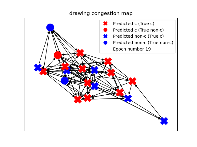
To illustrate how this dataset can be used in the context of traffic prediction, we have made an experiment using a graph neural network (GNN) that predicts node congestion. In this experiment we trained a GNN model on a dataset generated by S-RoadGNN to predict whether a node is congested or not. We included in Figure 3 a graphical representation of the prediction results of the GNN. Figure 3 shows the resulting predictions for a single example graph after twenty epochs of training. This experiment was run using a Graph Attention Network (GAT) with three layers. The training dataset contained 100 graphs of 20 nodes, while the validation set contained 40 graphs of 20 nodes. The specific graph that is drawn in Figure 3 was drawn randomly from the validation set. In this figure, the model correctly predicted congestion in of the nodes.
6 Conclusion
We motivate and present road data models, some of their theoretical properties and a tool, called TØIRoads, for generating datasets within these models. While one may be tempted to assume that preventing congestion is always desirable, this may not be the case if congestion of non-environmental friendly means of transportation, such as private cars, serve as incentive for the use of public transportation. Nevertheless, being able to study the scenarios related to changes in the population and traffic flow depending on points of interest and to predict congestion (whether to prevent it or not) is important for long-term city planning. As future work, we plan to include a few more parameters such as a sensible strategy for adding location information (currently only represented in a relative way, based on paths and their weights) to our road data models. A potential improvement would be to allow different densities per region of the graph, to simulate more dense districts, as commonly happens to districts that are close to the center of a city.
References
- [1] Azzedine Boukerche, Yanjie Tao, and Peng Sun. Artificial intelligence-based vehicular traffic flow prediction methods for supporting intelligent transportation systems. Comput. Networks, 182:107484, 2020. doi:10.1016/j.comnet.2020.107484.
- [2] Azzedine Boukerche and Jiahao Wang. Machine learning-based traffic prediction models for intelligent transportation systems. Comput. Networks, 181:107530, 2020. doi:10.1016/j.comnet.2020.107530.
- [3] Khac-Hoai Nam Bui, Jiho Cho, and Hongsuk Yi. Spatial-temporal graph neural network for traffic forecasting: An overview and open research issues. Appl. Intell., 52(3):2763–2774, 2022. doi:10.1007/s10489-021-02587-w.
- [4] Khac-Hoai Nam Bui, Hongsuk Yi, and Jiho Cho. UVDS: A new dataset for traffic forecasting with spatial-temporal correlation. In Ngoc Thanh Nguyen, Suphamit Chittayasothorn, Dusit Niyato, and Bogdan Trawinski, editors, Intelligent Information and Database Systems - 13th Asian Conference, ACIIDS 2021, Phuket, Thailand, April 7-10, 2021, Proceedings, volume 12672 of Lecture Notes in Computer Science, pages 66–77. Springer, 2021. doi:10.1007/978-3-030-73280-6_6.
- [5] Jeongwhan Choi and Noseong Park. Graph neural rough differential equations for traffic forecasting. ACM Trans. Intell. Syst. Technol., 14(4):74:1–74:27, 2023. doi:10.1145/3604808.
- [6] Zhiyong Cui, Ruimin Ke, Ziyuan Pu, Xiaolei Ma, and Yinhai Wang. Learning traffic as a graph: A gated graph wavelet recurrent neural network for network-scale traffic prediction. Transportation Research Part C: Emerging Technologies, 115:102620, 2020. doi:10.1016/j.trc.2020.102620.
- [7] Austin Derrow-Pinion, Jennifer She, David Wong, Oliver Lange, Todd Hester, Luis Perez, Marc Nunkesser, Seongjae Lee, Xueying Guo, Brett Wiltshire, Peter W. Battaglia, Vishal Gupta, Ang Li, Zhongwen Xu, Alvaro Sanchez-Gonzalez, Yujia Li, and Petar Velickovic. ETA prediction with graph neural networks in google maps. In Gianluca Demartini, Guido Zuccon, J. Shane Culpepper, Zi Huang, and Hanghang Tong, editors, CIKM ’21: The 30th ACM International Conference on Information and Knowledge Management, Virtual Event, Queensland, Australia, November 1 - 5, 2021, pages 3767–3776. ACM, 2021. doi:10.1145/3459637.3481916.
- [8] Alessio Gravina and Danilo Numeroso. NumGraph. https://numgraph.readthedocs.io.
- [9] Xiao Han, Guojiang Shen, Xi Yang, and Xiangjie Kong. Congestion recognition for hybrid urban road systems via digraph convolutional network. Transportation Research Part C: Emerging Technologies, 121:102877, 2020. doi:10.1016/j.trc.2020.102877.
- [10] Andreas Horni, Kai Nagel, and Kay Axhausen. Introducing MATSim, pages 3–8. Ubiquity Press, August 2016. doi:10.5334/baw.1.
- [11] Weiwei Jiang and Jiayun Luo. Graph neural network for traffic forecasting: A survey. Expert Syst. Appl., 207:117921, 2022. doi:10.1016/j.eswa.2022.117921.
- [12] Weiwei Jiang, Jiayun Luo, Miao He, and Weixi Gu. Graph neural network for traffic forecasting: The research progress. ISPRS Int. J. Geo Inf., 12(3):100, 2023. doi:10.3390/ijgi12030100.
- [13] Alexandra Kapp, Julia Hansmeyer, and Helena Mihaljevic. Generative models for synthetic urban mobility data: A systematic literature review. ACM Comput. Surv., 56(4):93:1–93:37, 2024. doi:10.1145/3610224.
- [14] Yaguang Li, Rose Yu, Cyrus Shahabi, and Yan Liu. Diffusion convolutional recurrent neural network: Data-driven traffic forecasting. In 6th International Conference on Learning Representations, ICLR 2018, Vancouver, BC, Canada, April 30 - May 3, 2018, Conference Track Proceedings. OpenReview.net, 2018. URL: https://openreview.net/forum?id=SJiHXGWAZ.
- [15] Jiaqi Ma, Jiong Zhu, Yuxiao Dong, Danai Koutra, Jingrui He, Qiaozhu Mei, Anton Tsitsulin, Xingjian Zhang, and Marinka Zitnik. The 3rd workshop on graph learning benchmarks (GLB 2023). In Ambuj K. Singh, Yizhou Sun, Leman Akoglu, Dimitrios Gunopulos, Xifeng Yan, Ravi Kumar, Fatma Ozcan, and Jieping Ye, editors, Proceedings of the 29th ACM SIGKDD Conference on Knowledge Discovery and Data Mining, KDD, pages 5870–5871. ACM, 2023. doi:10.1145/3580305.3599224.
- [16] Johannes Nguyen, Simon T. Powers, Neil Urquhart, Thomas Farrenkopf, and Michael Guckert. An overview of agent-based traffic simulators. Transportation Research Interdisciplinary Perspectives, 12:100486, 2021. doi:10.1016/j.trip.2021.100486.
- [17] Eren Olug, Kiymet Kaya, Resul Tugay, and Sule Gündüz Ögüdücü. IBB traffic graph data: Benchmarking and road traffic prediction model. CoRR, abs/2408.01016, 2024. doi:10.48550/arXiv.2408.01016.
- [18] Chao Song, Youfang Lin, Shengnan Guo, and Huaiyu Wan. Spatial-temporal synchronous graph convolutional networks: A new framework for spatial-temporal network data forecasting. In AAAI, pages 914–921. AAAI Press, 2020. doi:10.1609/aaai.v34i01.5438.
-
[19]
Grunde Haraldsson Wesenberg.
gruwesen/TOIROADS.
Software, version 1.0., Norwegian Research Council, project 322480,
swhId:
swh:1:dir:a86388944844fcc00f4cad67e1ec75a99
8f36eae (visited on 2024-12-11). URL: https://github.com/gruwesen/TOIROADS, doi:10.4230/artifacts.22621. - [20] Bing Yu, Haoteng Yin, and Zhanxing Zhu. Spatio-temporal graph convolutional networks: A deep learning framework for traffic forecasting. In Jérôme Lang, editor, Proceedings of the Twenty-Seventh International Joint Conference on Artificial Intelligence, IJCAI 2018, July 13-19, 2018, Stockholm, Sweden, pages 3634–3640. ijcai.org, 2018. doi:10.24963/ijcai.2018/505.